"Why Should I Trust You?": Explaining the Predictions of Any Classifier
Introduction
Understanding why machine learning models behave the way they do helps users in model selection, feature engineering, and finally trusting the model to deploy it. In many cases even though a non-interpretable model is more accurate on the validation data set than the interpretable one, an interpretable model is chosen. But restricting the models to just an interpretable model isn't the best option. In this paper, the authors argue for explaining machine learning predictions using model-agnostic approaches and propose LIME (Local Interpretable Model-Agnostic Explanations), a novel explanation technique that explains the predictions of any classifier in an interpretable and faithful manner, by learning an interpretable model locally around the prediction. They also propose a method called sub-modular optimization to explain models globally by selecting a representative individual prediction.
Some recent work aims to anticipate failures in machine learning, specifically for vision tasks. Failure modes are found by grouping incorrectly classified images according to a semantic attribute space, which are descriptions explaining the cause of the failure [12]. Another approach is to train a model that can predict failure [14]. Letting users know when the systems are likely to fail can lead to an increase in trust, by avoiding “silly mistakes” [13]. These solutions either require additional annotations and feature engineering that is specific to vision tasks or do not provide insight into why a decision should not be trusted. Furthermore, they assume that the current evaluation metrics are reliable, which may not be the case if problems such as data leakage are present. This is not the first work to look at the problems with relying on validation set accuracy as the primary measure of trust. This area has been well studied. Practitioners often overestimate their model's accuracy, propagate feedback loops, and fail to notice data leaks. Common solutions in the literature are Gestalt and Modeltracker. The LIME technique complements these tools.
The experiments are conducted mainly on text data and image data, where models used are Random Forest (RF) and Convolutional Neural Networks (CNN). The experiments highlight utility of explanations in deciding between the models, which model is to be trusted and which is not and also improving the model based on the explanations. The main contributions of this paper are summarized as follows.
- LIME, an algorithm to explain any prediction of any model (classifier or regressor) by approximating locally with an interpretable model that is faithful to the original model locally.
- SP-LIME, a method to select a final set of representative samples using sub-modular optimization to show to the user that pretty much captures what the original model is doing globally.
- A detailed set of experiments with simulated subjects to prove the usefulness of LIME and SP-LIME.

Need for Explanations
Prediction explanation basically means answering question such as "What triggers the model to make such a prediction?", and an answer to that would be to say, these are the features with a certain range of values in your input sample that are contributing to the prediction the most. For example, it can be words in a document for text classification or patches of pixels in an image for image classification. And these explanations need to make sense to the user and hence has to be simple. Figure 1 illustrates an explanation procedure. In this case, an explanation is a small weighted list of symptoms that either contribute to the prediction (in green) or are evidence against it (in red). It is very clear that the life of a doctor is much easier in terms of making a decision with the help of a model if intelligible explanations are provided. This is similar to the topic of inference versus prediction. Some people tend to think of these two terms are the same. However, statistically, their meanings are very different. Inference means given some datasets, we would like to infer how the output/response is generated based on a sequence of explanatory variables. For instance, we would like to know/infer how education level affects people’s income level. Prediction, on the other hand, is by using a given dataset, we fit/train a model that will correctly predict the outcome of a new observation.
Even with highest accuracy on validation dataset, we sometimes can't judge how the model is going to behave on other datasets. There are many reasons why this can happen. For example, Data leakage where some of the features used for training are heavily correlated with the target value in both training and validation data that might result in great train and validation results but will be of no use if used on altogether a new dataset. But if explanations such as the one in Figure 1 are given, it becomes easy to fix the fault by removing the heavily correlated feature from the data and train. This is how you convert an untrustworthy model to a trustworthy one. Another problem is dataset shift, where train and test data come from different distributions and providing explanations for predictions will help the user to take measures to make model generalize better.
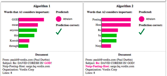
Figure 2 shows how explanations help in selecting between the models in addition to accuracy measures. In this case, by looking at the explanations it is easy to say that model with higher accuracy is in-fact the worst. Further, many a times, there can be difference between what we want the model to optimize and what the model is actually optimizing which might result into model not behaving as well as expected (For example in binary classification using logistic regression, all we are concerned is with accuracy, but the model is trying to reduce the log-loss due to the learning algorithms limitations). While we may not be able to quantitatively measure what difference has that made, but we still have some intuitions as to how the model has to behave with respect to some of its features, and if explanations are given for model predictions, we will be able to ascertain if those explanations make any sense. Also explaining models being model agnostic helps as we then compare different classes of models in making a choice.
Desired Characteristics for Explainers
Explainers have to be simple models so that humans are able to comprehend what the model is doing. For example, even with linear models, if the number of features are too many, it becomes hard for humans to comprehend an overwhelming set of features. In case of models trained with word-embedding as features, we can't give these word-embeddings as explanations, instead, they need to something different than these features.
Another requirement of a good explainer is that it has to be locally faithful to the original model, i.e, it must behave similarly to the model in the vicinity of the instance being predicted. And these local explanations should aid in forming global explanations.
Desired Characteristics for Explanations
Interpretable(understanding between the input and response)
- Take into account user limitations.
- Since features in a machine learning model need not be interpretable, the input to the explanations may have to be different from input to the model.
Local Fidelity
- Explanation should be locally faithful, ie it should correspond to how the model behaves in the vicinity of the instance being predicted. It doesn't mean global fidelity, where global important features may not be important in the local context.
Model Agnostic
- Treat the original, given model as a black box.
Global Perspective (explain the model)
- Select a few predictions such that they represent the entire model.
Local Interpretable Model-Agnostic Explanations (LIME)
The overall goal of LIME is to basically identify an interpretable model over the interpretable representation (features) that is locally faithful to the classifier. Here, interpretable explanations need to use a representation that is understandable to humans, regardless of the actual features used by the model. For example in case of text classification, a possible interpretable representation of data would be to use bag of words (one-hot encodings) instead of the word embeddings. Similarly, for image classification, it may be a binary vector (one-hot encoding) indicating the “presence” or “absence” of a contiguous patch of pixels (a super-pixel or a segment), while the classifier may represent the image as a tensor with three color channels per pixel. Let $x ∈ R^d$ be the original representation of an instance being explained, and $x' ∈ \{0, 1\}^{d'}$ be a binary vector for its interpretable representation.
Fidelity-Interpretability Trade-Off
Formally, the authors define an explanation as a model $g ∈ G$, where $G$ is a class of potentially interpretable models, such as linear models, decision trees, or falling rule lists [3]. The domain of $g$ is $\{0, 1\}^{d'}$, i.e. $g$ acts over absence/presence of the interpretable components. Let $Ω(g)$ be a measure of complexity (like a regularizer term) of the explanation $g ∈ G$. For example, for decision trees $Ω(g)$ may be the depth of the tree, for linear models, $Ω(g)$ may be the number of non-zero weights. Let the model being explained be denoted $f : R^d → R$. In classification, $f(x)$ is the probability that $x$ belongs to a certain class. We further use $π_x(z)$ as a proximity measure between an instance $z$ to $x$, so as to define locality around $x$. Finally, let $L(f, g, π_x)$ be a measure of error between $g$ and $f$ in the locality defined by $π_x$. Our task is to minimize $L(f, g, π_x)$ while having $Ω(g)$ be low enough to be interpretable by humans. The minimum value of $L(f, g, π_x)$ provides an approximate balance measure for preserving interpretability and local fidelity(it should correspond to how the model behaves in the vicinity of the instance being predicted). The explanation produced by LIME is obtained by the following:
- [math]\displaystyle{ \xi(x) = \underset{g\in\mathbb{G}}{\operatorname{argmin}}\, \mathcal{L}(f,g,\pi_x) + \Omega(g)\,\,\,\,\,\,\,\,\,\,\,\,\,\,\, Eq. (1) }[/math]
Even though $G$ can be any class of interpretable models, in this paper only sparse linear models are considered.
Sampling for Local Exploration
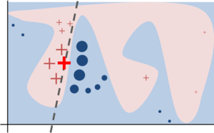
The aim is to minimize $L(f, g, π_x)$ without making any assumptions about $f$, since the explainer needs to be model-agnostic. In order to learn the local behavior of $f$ using $g$ as the interpretable inputs vary, $L(f, g, π_x)$ is approximated by drawing samples, weighted by $π_x$. We sample instances around $x'$ by setting few features of $x'$ to 0, uniformly at random (where the number of such features set to 0 is also uniformly sampled). Given a perturbed sample $z' ∈ \{0, 1\}^{d'}$ (which contains a fraction of the features of $x'$ set to 0), we recover the sample in the original representation $z ∈ R^d$ and obtain the prediction $f(z)$ from the original classifier, and is used as a label for the explanation model. Given this dataset $Z$ of perturbed samples with the associated labels, we optimize Eq. (1) to get an explanation $ξ(x)$. The primary intuition behind LIME is presented in Figure 3, where we sample instances both in the vicinity of $x$ (which have a high weight due to $π_x$) and far away from $x$ (low weight from $π_x$). Even though the original model may be too complex to explain globally, LIME presents an explanation that is locally faithful (linear in this case), where the locality is captured by a weight factor, $π_x$. A concrete example of this process is presented in the next section.
Sparse Linear Explanations
For the rest of this paper, we let $G$ be the class of linear models, such that $g(z') = w_g · z'$ . We use the locally weighted square loss as $L$, as defined in Eq. (2), where we let $π_x(z) = exp(−D(x, z)^2 /σ^2 )$ be an exponential kernel defined on some distance function $D$ (e.g. cosine distance for text, L2 distance for images) with width $σ$ resulting in higher sample weights for perturbed samples that are in the vicinity of sample being explained and lower weights for samples that are far away.
- [math]\displaystyle{ \mathcal{L}(f,g,\pi_x) = \underset{z,z'\in\mathbb{Z}}{\operatorname{\Sigma}} \pi_x(z)\,(f(z) - g(z'))^2\,\,\,\,\,\,\,\,\,\,\,\, Eq.(2) }[/math]
For text classification, the features used for explanation models are bag of words, and we set a limit on the number of words used for explanation, $K$. i.e. $Ω(g) = ∞1[||w_g||_0 > K]$. We use the same $Ω$ for image classification, using “super-pixels” (computed using any standard image segmentation algorithm, eg. quickshift() function in skimage python library [5]) instead of words, such that the interpretable representation of an image is a binary vector where 1 indicates the original super-pixel and 0 indicates a grayed out super-pixel. This particular choice of $Ω$ makes directly solving Eq. (1) intractable, but we approximate it by first selecting $K$ features with Lasso (using the regularization path [4]) (scikit lars_path method [6]) and then learning the weights via least squares (together a procedure we call K-LASSO in Algorithm 1). .
There are some limitations to class of locally interpretable models $G$. It can happen that no $g \in G$ is powerful enough to be locally faithful to the original model, i.e, $g$ has a high bias w.r.t $f$ locally. This may be because the underlying model is quite complex even locally. Another issue could be, the features used for building explanations are not representative of the inputs or factors that the underlying model relies on. For example, a model that predicts sepia-toned images to be retro cannot be explained by the presence or absence of super pixels.
Examples
Example 1: Text classification with SVMs
In Figure 2 (right side), LIME explains an SVM classifier with RBF kernel trained on "20 newsgroup dataset" to classify documents into "Atheism" and "Christianity". Even though it achieves 94% accuracy on validation dataset, the explanation for an instance shows that features that are used the most in predictions are very arbitrary such as words like "Posting", "Host" and "Re", which have no connection to either Christianity or Atheism. Even if these stop words or headers are removed, the classifier still considers the proper names of people writing the post to be important features, which clearly doesn't make sense. Hence we can conclude by looking at the explanations that the dataset has serious issues and when a classifier is trained on it, it won't be able to generalize well. Hence suitable steps needed to be taken to train a trustworthy classifier.
Example 2: Deep networks for images
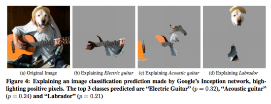
In this example, we use sparse linear explanations to explain Google’s pre-trained Inception neural network [7] which is an image classifier. Here features used for giving explanations are super-pixels (segments) which intuitively makes sense as we humans detect an object in an image based on certain parts of the object. Figure 4a show an arbitrary image that we want to explain. Figures 4b, 4c, 4d show the super-pixels that contribute the most while predicting the image to be one of the top 3 classes. Here we set max feature count for explainer, $K = 10$. It is quite intuitive from Figure 4b in particular that why acoustic guitar was predicted to be an electric based on the fretboard that resembles an acoustic guitar. So even though the prediction is incorrect, it still is not unreasonable at all.
Submodular Pick for Explaining Models
Submodular pick provides some sort of a global understanding of the model by methodically picking a set of non-redundant sample explanations. This method is still model agnostic and complimentary to calculating validation accuracy in machine learning problem. If we choose a large number of instances to explain, the user may not be able to go through each of them and verify what is wrong or right with the model. We say humans have a budget $B$, that is the number of instance explanations that they are willing to examine. So given a set of $X$ instances, the task of sub-modular optimization is to pick a maximum of $B$ instances that effectively capture the essence of what the model is doing in a non-redundant way.
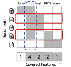
Here we have a explanations for $n$ instances and we construct an $n × d'$ matrix $W$, each row of which represent local importances of features used for each instance explanations. In case of using sparse linear models as explanations, for an instance $x_i$ and explanation $g_i = ξ(x_i)$, we set $W_{ij} = |w_{gij}|$. Further, for each feature (column) $j$ in $W$, let $I_j$ denote the global importance of that component in the explanation space. Intuitively, $I$ represents global importance of each feature. In Figure 5, we show a toy example $W$, with $n = d' = 5$, where $W$ is binary (for simplicity). Since feature $f2$ is used in most of the explanations, $I$ should have higher value for feature $f2$ than $f1$, i.e. $I_2 > I_1$. Formally for the text classifiers, we set $I_j = \sqrt{\sum_{i=1}^nW_{ij}}$ . For images, $I$ must represent something that can be compared across the super-pixels (segments) in different images, such as color histograms or other features of super-pixels; But this is left as a future work for now.
While picking the samples, we must be careful in not picking up samples that explain the same thing. So we want a minimum set of samples that cover the maximum number of features as possible. In Figure 5, after the second row is picked, the third row is redundant, as the user has already seen features $f2$ and $f3$ - while the last row gives the user completely new features. Hence selecting the second and last row results in giving the maximum coverage of features. Eq. (3) formalizes this process, where we define coverage as the set function $c$ that, given $W$ and $I$, computes the total importance of the features that at least appear in one instance in a set $V$ .
- [math]\displaystyle{ c(V, W, I) = {{\sum_{j = 1}^{d'}}}\mathbb{1}_{[\exists i\in V:W_{ij}\gt 0]}I_j\,\,\,\,\,\,\,\,\,\,\,\,\,\,\, Eq. (3) }[/math]
The pick problem, defined in Eq. (4), consists of finding the set $V, |V| ≤ B$ that achieves the highest coverage.
- [math]\displaystyle{ Pick(W, I) = \underset{V,|V|\leq B}{\operatorname{argmax}}\, c(V,W, I)\,\,\,\,\,\,\,\,\,\,\,\,\,\,\, Eq. (4) }[/math]
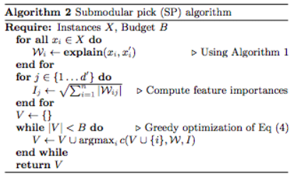
The problem in Eq. (4) is maximizing a weighted coverage function, and is NP-hard [10]. Let $c(V\cup\{i\}, W, I)−c(V, W, I)$ be the marginal coverage gain of adding an instance $i$ to a set $V$ . Due to sub-modularity, a greedy algorithm that iteratively adds the instance with the highest marginal coverage gain to the solution offers a constant-factor approximation guarantee of $1−1/e$ to the optimum [8]. This approximation process is outlined in Algorithm 2 and is called sub-modular pick.
Simulated User Experiments
This section highlights simulated user experiments conducted to evaluate how explanations help the user in different tasks. In particular, following questions are addressed: (1) Are the explanations faithful to the model, that is are the explainers correctly highlighting the important features that the model is selecting at least locally? (2) Can the explanations help users in ascertaining trust in predictions; that is to say, if the predictions make sense or not? and (3) Are the explanations useful for evaluating the model as a whole and thereby aid in finally selecting a model? Code and data for experiments are available at https://github.com/marcotcr/lime-experiments.
Experiment Setup
2 sentiment analysis datasets (books and DVDs, 2000 instances each) where the task is to classify product reviews as positive or negative [9] are used in the experiment. Decision trees (DT), logistic regression with L2 regularization (LR), nearest neighbors (NN), and SVMs with RBF kernel, all using bag of words as features are trained separately. There is also a random forest (with 1000 trees) trained over average word2vec embeddings (RF). Unless otherwise noted, default methods of scikit are used. Dataset is divided into train and test in the ratio of 4:1. To explain individual predictions, LIME is compared with parzen [10], a method that approximates the black box classifier globally with Parzen windows, and explains individual predictions by taking the gradient of the prediction probability function. (Parzen-window density estimation is essentially a data-interpolation technique. Given an instance of the random sample, ${\bf x}$, Parzen-windowing estimates the PDF $P(X)$ from which the sample was derived. It essentially superposes kernel functions placed at each observation or datum. In this way, each observation $x_i$ contributes to the PDF estimate [15]). For parzen, $K$ features are selected as explanations such that they have the highest absolute gradients. Hyper-parameters for LIME and parzen are set using cross-validations and number of perturbed samples for a single explanation, $N$ is set to 15000. There is also a comparison made against a greedy procedure in which features that contribute the most to the predicted class are greedily removed until prediction changes or we reach a maximum of $K$ features that are removed, and these $K$ or fewer features are finally selected to explain the model. Also a random procedure that randomly picks K features as an explanation is also used for comparison. For all the experiments below $K$ is set to 10. For experiments where the pick procedure applies, it's either a random pick (RP) or sub-modular pick (SP). We refer to pick-explainer combinations by adding RP or SP as a prefix.
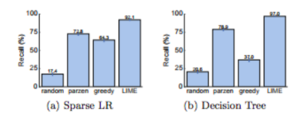
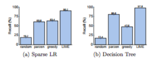
Are explanations faithful to the model?
Here we evaluate faithfulness of explanations on classifiers that are by themselves explicable such as sparse logistic regression or decision trees. So we train 2 models, a sparse logistic regressor and a decision tree such that the maximum number of features they use 10 so we now know what the important features (gold features) really are for these 2 models. For each prediction on the test set, we generate explanations and compute the fraction of these gold features that are recovered by the explanations (recall). We report this recall averaged over all the test instances in Figures 6 and 7. From the bar graphs we can see that the greedy approach is comparable to parzen on logistic regression, but is substantially worse on decision trees since changing a single feature at a time often does not have an effect on the prediction. The overall recall by parzen is low, likely due to the difficulty in approximating the original high-dimensional classifier. LIME consistently provides > 90% recall for both classifiers on both datasets, and this demonstrates that LIME explanations are more faithful to the model than any other explanations.
Should I trust this prediction?
In order to simulate trust in individual predictions, we first randomly select 25% of the features to be “untrustworthy”, and assume that the users can identify and would not want to trust these features (such as the headers in 20 newsgroups, leaked data, etc). We thus develop oracle “trustworthiness” by labeling test set predictions from a black box classifier as “untrustworthy” if the prediction changes when untrustworthy features are removed from the instance, and “trustworthy” otherwise. In order to simulate users, we assume that users deem predictions untrustworthy from LIME and parzen explanations if the prediction from the linear approximation changes when all untrustworthy features that appear in the explanations are removed (the simulated human “discounts” the effect of untrustworthy features). For greedy and random, the prediction is mistrusted if any untrustworthy features are present in the explanation since these methods do not provide a notion of the contribution of each feature to the prediction. Thus for each test set prediction, we can evaluate whether the simulated user trusts it using each explanation method, and compare it to the trustworthiness oracle.
Using this setup, we report the score, F1 (average of precision and recall) on the trustworthy predictions for each explanation method, averaged over 100 runs, in Table 1. The results indicate that LIME dominates others (all results are significant at p = 0.01) on both datasets, and for all of the black box models. The other methods either achieve a lower recall (i.e. they mistrust predictions more than they should) or lower precision (i.e. they trust too many predictions), while LIME maintains both high precision and high recall. Even though we artificially select which features are untrustworthy, these results indicate that LIME is helpful in assessing trust in individual predictions.

Can I trust this model?
In the final simulated user experiment, we consider a case where the user has to pick between 2 competing models with similar accuracy on validation dataset. For this purpose, we add 10 artificially “noisy” features. Specifically, on training and validation sets (80/20 split of the original training data), each artificial feature appears in 10% of the examples in one class, and 20% of the other, while on the test instances, each artificial feature appears in 10% of the examples in each class. This recreates the situation where the models use not only features that are informative in the real world, but also ones that introduce spurious correlations. We create pairs of competing classifiers by repeatedly training pairs of random forests with 30 trees until their validation accuracy is within 0.1% of each other, but their test accuracy differs by at least 5%. Thus, it is not possible to identify the better classifier (the one with higher test accuracy) from the accuracy on the validation data.
The goal of this experiment is to evaluate whether a user can identify the better classifier based on the explanations of $B$ instances from the validation set. The simulated human marks the set of artificial features that appear in the $B$ explanations as untrustworthy, following which we evaluate how many total predictions in the validation set should be trusted (as in the previous section, treating only marked features as untrustworthy). Then, we select the classifier with fewer untrustworthy predictions and compare this choice to the classifier with higher held-out test set accuracy.
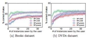
We present the accuracy of picking the correct classifier as $B$ varies, averaged over 800 runs, in Figure 8. We omit SP-parzen and RP-parzen from the figure since they did not produce useful explanations, performing only slightly better than random. LIME is consistently better than greedy, irrespective of the pick method. Further, combining sub-modular pick with LIME outperforms all other methods, in particular, it is much better than RP-LIME when only a few examples are shown to the users. These results demonstrate that the trust assessments provided by SP-selected LIME explanations are good indicators of generalization.
Conclusion and Future Work
The paper evaluates its approach on a series of simulated and human-in-the-loop tasks to check:
- The predictions of any classifier in an interpretable and faithful manner.
- The method to explain its models by obtaining individual predictions and their explanations.
- Could the predictions be trusted.
- Can the model be trusted.
- Can users select the best classifier given the explanations.
- Can user (non-experts) improve the classifier by means of feature selection.
- Can explanations lead to insights about the model itself.
This paper successfully argues for the importance of explaining the predictions to make the model more trustworthy to the user. It proposes LIME, a comprehensive approach to faithfully explain predictions of any model in the simplest way desired. Detailed experiments demonstrating how explanations helped users pick models or discard models are provided. As a future consideration, authors want to repeat the experiments with decision trees being the interpretable model instead of sparse linear models. Authors also want to come up with an approach to perform the pick step for images. They also want to look into an automated way of selecting hyper-parameters used in LIME and SP-LIME such as K, N etc. and finally consider running the code on GPU to create explanations in real-time.
Remarks and Critique
This paper is by far the best paper I have read on model interpretability. The paper is full of new ideas and the authors clearly explain the approaches used with reasons as to why they picked it and also highlight both weaknesses and strong points of the approaches. Even though some of the tricks used are a little ambiguous on paper such as K-Lasso, super-pixels, but going through the code on GitHub, it becomes more clear. The code is also very well documented and easy to install and run to reproduce the results published. I tried running it on CIFAR-10 dataset and found it to be useful in understanding my model better.
There are few minor details that are unanswered in the paper.
- To interpret prediction for an image classifier, authors use super-pixels (segments) as features, but they don't give any reason as to why they picked this approach. One of the reasons I can think of is that convolutional neural networks learn shapes from layer to layer, which becomes more and more complete as we move from top to lower layers. So in a way you can say, the classifier classifies on the basis of set of groups of pixels close to each other (as in the case of segments) than just the pixels that are spread apart far away from each other.
- The authors don't say how locally faithful the interpretable model should be to the classifier with constraints on the maximum number of features to be used, i.e, what is the sort of error (mean squared error in case of linear interpretable models) we are content with?
- It seems that LIME can easily extended to regression cases and is not just limited to classification tasks, but the paper doesn't discuss anything in this regard.
This paper is also comparable to the DeepLIFT[17] method, which provides a global numerical recovery of sample manifold. Both methods rely heavily on the reference point chosen. LIME has the advantage of matching the behavior of the model with interpretable explanations, while DeepLIFT focuses on the model structure and yields overall assessment of the model by manually feeding several typical reference inputs into the method.
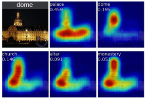
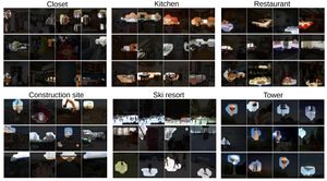
In this paper, the experiments with Deep Convolutional Neural Network try to find the pixels which contribute most to the final output. As a complement reference, this paper[16] also focuses on the interpretability of CNN models by sharing the same idea. In that work, the authors use Global Averaging Pooling layer after the last convolutional layer. Then a heat map is generated by a weighted sum of the outputs from last convolutional layer. By plugging back to the input image, the area that contributes most to the output is highlighted.
-
Figure 9: example output from CAM
-
Figure 10: example output from CAM
As a result, we can actually tell what is the model learning. Examples are shown in Figure 9, 10.
References
[1] Marco Tulio Ribeiro, Sameer Singh, Carlos Guestrin, Model-Agnostic Interpretability of Machine Learning, presented at 2016 ICML Workshop on Human Interpretability in Machine Learning (WHI 2016), New York, NY
[2] Marco Tulio Ribeiro, Sameer Singh, Carlos Guestrin, “Why Should I Trust You?” Explaining the Predictions of Any Classifier, KDD 2016 San Francisco, CA, USA
[3] F. Wang and C. Rudin. Falling rule lists. In Artificial Intelligence and Statistics (AISTATS), 2015.
[4] B. Efron, T. Hastie, I. Johnstone, and R. Tibshirani. Least angle regression. Annals of Statistics, 32:407–499, 2004.
[5] http://scikit-image.org/docs/dev/api/skimage.segmentation.html#skimage.segmentation.quickshift
[6] http://scikit-learn.org/stable/modules/generated/sklearn.linear_model.lars_path.html
[7] C. Szegedy, W. Liu, Y. Jia, P. Sermanet, S. Reed, D. Anguelov, D. Erhan, V. Vanhoucke, and A. Rabinovich. Going deeper with convolutions. In Computer Vision and Pattern Recognition (CVPR), 2015.
[8] A. Krause and D. Golovin. Submodular function maximization. In Tractability: Practical Approaches to Hard Problems. Cambridge University Press, February 2014.
[9] J. Blitzer, M. Dredze, and F. Pereira. Biographies, bollywood, boom-boxes and blenders: Domain adaptation for sentiment classification. In Association for Computational Linguistics (ACL), 2007.
[10] D. Baehrens, T. Schroeter, S. Harmeling, M. Kawanabe, K. Hansen, and K.-R. Muller. How to explain individual classification decisions. Journal of Machine Learning Research, 11, 2010.
[11] https://en.wikipedia.org/wiki/Precision_and_recall
[12] A. Bansal, A. Farhadi, and D. Parikh. Towards transparent systems: Semantic characterization of failure modes. In European Conference on Computer Vision (ECCV), 2014.
[13] M. T. Dzindolet, S. A. Peterson, R. A. Pomranky, L. G. Pierce, and H. P. Beck. The role of trust in automation reliance. Int. J. Hum.-Comput. Stud., 58(6), 2003.
[14] P. Zhang, J. Wang, A. Farhadi, M. Hebert, and D. Parikh. Predicting failures of vision systems. In Computer Vision and Pattern Recognition (CVPR), 2014.
[15] Parzen Density Windows :- https://www.cs.utah.edu/~suyash/Dissertation_html/node11.html
[16] Zhou, Bolei et al. “Learning Deep Features for Discriminative Localization.” 2016 IEEE Conference on Computer Vision and Pattern Recognition (CVPR) (2016): 2921-2929.
[17] Avanti Shrikumar, Peyton Greenside, Anshul Kundaje: Learning Important Features Through Propagating Activation Differences (link)
