stat841f10

Classfication-2010.09.21

Classification

Statistical classification, usually simply known as classification, is an area of supervised learning that addresses the problem of how to systematically assign unlabeled novel data to their labels (also known as classes or groups) by using knowledge of their features (also known as characteristics or attributes) that are obtained from observation and/or measurement. A classifier is a specific technique or methodology for performing classification. To classify new data, a classifier first uses labeled training data to train a model, and then it uses a classification rule to assign labels to the new data based on prediction results given by the model.

Classification is an important task for people and society since the beginnings of history. According to this link, the earliest application of classification in human society was probably done by prehistory peoples for recognizing which wild animals were beneficial to people and which one were harmful, and the earliest systematic use of classification was done by the famous Greek philosopher when he, for example, divided all living things into the two groups of plants and animals. Classification is generally regarded as one of four major areas of statistics, with the other three major areas being regression regression, clustering, and dimensionality reduction (also known as feature extraction or manifold learning).

In classical statistics, classification techniques were developed to learn useful information using small data sets where there is usually not enough of data. When machine learning was developed after the application of computers to statistics, classification techniques were developed to work with very large data sets where there is usually too many data. A major challenge facing data mining using machine learning is how to efficiently find useful patterns in very large amounts of data. A interesting quote that describes this problem quite well is the following one made by the retired Yale University Librarian Rutherford D. Rogers.

       "We are drowning in information and starving for knowledge."  
                                                         - Rutherford D. Rogers

In the Information Age, machine learning when it is combined with efficient classification techniques can be very useful for data mining using very large data sets. This is most useful when the structure of the data is not well understood but the data nevertheless exhibit strong statistical regularity. Areas in which machine learning and classification have been used together include search and recommendation (e.g. Google, Amazon),automatic speech recognition and speaker verification, medical diagnosis, analysis of gene expression, drug discovery etc.

The formal mathematical definition of classification is as follows:

Definition: Classification is the prediction of a discrete random variable [math]\displaystyle{ \mathcal{Y} }[/math] from another random variable [math]\displaystyle{ \mathcal{X} }[/math].

A set of training data used by a classifier to train a model consists of [math]\displaystyle{ \,n }[/math] independently and identically distributed (i.i.d) ordered pairs [math]\displaystyle{ \,\{(X_{1},Y_{1}), (X_{2},Y_{2}), \dots , (X_{n},Y_{n})\} }[/math], where the values of the [math]\displaystyle{ \,ith }[/math] training input's attributes [math]\displaystyle{ \,X_{i} = (\,X_{i1}, \dots , X_{id}) \in \mathcal{X} \subset \mathbb{R}^{d} }[/math] is a d-dimensional vector and the label of the [math]\displaystyle{ \, ith }[/math] training input is [math]\displaystyle{ \,Y_{i} \in \mathcal{Y} }[/math] that takes a finite number of values. The classification rule used by a classifier has the form [math]\displaystyle{ \,h: \mathcal{X} \mapsto \mathcal{Y} }[/math]. After the model is trained, each new data input, the values of whose features is [math]\displaystyle{ \,X \in \mathcal{X}, }[/math] is labeled [math]\displaystyle{ \,\hat{Y}=h(X) \in \mathcal{Y} }[/math] using the classification rule [math]\displaystyle{ \,h: \mathcal{X} \mapsto \mathcal{Y} }[/math].

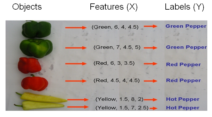
As an example, if we would like to classify some vegetables and fruits, then our training data might look something like the one shown in the following picture from Professor Ali Ghodsi's Fall 2010 STAT 841 slides.

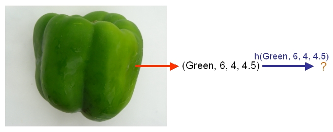
After we have selected a classifier and then built our model using the training data, we could use the classifier's classification rule [math]\displaystyle{ \,h: \mathcal{X} \mapsto \mathcal{Y} }[/math] to classify any newly-given vegetable or fruit such as the one shown in the following picture from Professor Ali Ghodsi's Fall 2010 STAT 841 slides after first obtaining the values of its features.

As another example, suppose we wish to classify newly-given fruits into apples and oranges by considering three features of a fruit that comprise its color, its diameter, and its weight. Then, after selecting a classifier and constructing a model using training data [math]\displaystyle{ \,\{(X_{\mathrm{color 1}}, X_{\mathrm{diameter 1}}, X{_\mathrm{weight 1}}, Y_{1}), (X_{2},Y_{2}), \dots , (X_{n},Y_{n})\} }[/math]

Linear and Quadratic Discriminant Analysis cont'd - 2010.09.23

In the second lecture, Professor Ali Ghodsi recapitulates that by calculating the class posteriors [math]\displaystyle{ \Pr(Y=k|X=x) }[/math] we have optimal classification. He also shows that by assuming that the classes have common covariance matrix [math]\displaystyle{ \Sigma_{k}=\Sigma \forall k }[/math] the decision boundary between classes [math]\displaystyle{ k }[/math] and [math]\displaystyle{ l }[/math] is linear (LDA). However, if we do not assume same covariance between the two classes the decision boundary is quadratic function (QDA).

Some MATLAB samples are used to demonstrated LDA and QDA

LDA x QDA

Linear discriminant analysis[1] is a statistical method used to find the linear combination of features which best separate two or more classes of objects or events. It is widely applied in classifying diseases, positioning, product management, and marketing research.

Quadratic Discriminant Analysis[2], on the other had, aims to find the quadratic combination of features. It is more general than Linear discriminant analysis. Unlike LDA however, in QDA there is no assumption that the covariance of each of the classes is identical.

Summarizing LDA and QDA

We can summarize what we have learned so far into the following theorem.

Theorem:

Suppose that [math]\displaystyle{ \,Y \in \{1,\dots,k\} }[/math], if [math]\displaystyle{ \,f_k(x) = Pr(X=x|Y=k) }[/math] is Gaussian, the Bayes Classifier rule is

[math]\displaystyle{ \,h(X) = \arg\max_{k} \delta_k(x) }[/math]

where

[math]\displaystyle{ \,\delta_k = - \frac{1}{2}log(|\Sigma_k|) - \frac{1}{2}(x-\mu_k)^\top\Sigma_k^{-1}(x-\mu_k) + log (\pi_k) }[/math] (quadratic)

• Note The decision boundary between classes [math]\displaystyle{ k }[/math] and [math]\displaystyle{ l }[/math] is quadratic in [math]\displaystyle{ x }[/math].

If the covariance of the Gaussians are the same, this becomes

[math]\displaystyle{ \,\delta_k = x^\top\Sigma^{-1}\mu_k - \frac{1}{2}\mu_k^\top\Sigma^{-1}\mu_k + log (\pi_k) }[/math] (linear)

• Note [math]\displaystyle{ \,\arg\max_{k} \delta_k(x) }[/math]returns the set of k for which [math]\displaystyle{ \,\delta_k(x) }[/math] attains its largest value.

Reference

The Elements of Statistical Learning: Data Mining, Inference, and Prediction

The Elements of Statistical Learning: Data Mining, Inference, and Prediction, Second Edition, February 2009 Trevor Hastie, Robert Tibshirani, Jerome Friedman

http://www-stat.stanford.edu/~tibs/ElemStatLearn/ (3rd Edition is available)