Robust Imitation Learning from Noisy Demonstrations

Presented by

Kar Lok Ng, Muhan (Iris) Li

Introduction

In Imitation Learning (IL), an agent (such as a neural network) aims to learn a policy from demonstrations of desired behaviour, so that it can make the desired decisions when presented with new situations. It differs from traditional Reinforcement Learning (RL), as it makes no assumption as to the nature of a reward function. IL methods assume that the demonstrations we feed the algorithm is optimal (or near optimal). This creates a big problem, as this method becomes very susceptible to poor data (i.e., not very robust). This intuitively makes sense, as the agent cannot effectively learn the optimal policy when it is fed low-quality demonstrations. As such, a robust method of IL is desired so that it can make better decisions despite being presented with noisy data. Established methods to combat noisy data in IL have limitations. One proposed solution requires the noisy demonstration to be ranked according to their relative performance to each other. Another similar method requires extra labelling of the data with a score that determines the probability that a particular demonstration is from an expert (a “good” demonstration). Both methods require extra data preprocessing that may not be feasible. A third method did not require these labels, but instead assume that noisy demonstrations were generated by a Gaussian distribution. This strict assumption limits the useability of such a model. Thus, a new method for IL from noisy demonstration is created. In this paper, they called this method Robust IL with Co-pseudo-labelling (RIL-Co). This method does not require additional labelling, nor does it require assumptions to be made about the noise distributions.

Model Architecture

On the basis of IL, the paper considers a scenario of replacing given demonstrations by a mixture of expert and non-expert demonstrations. Previously, the expert policy to be learned in IL is,

where [math]\displaystyle{ \rho_E }[/math] is a state-action density of expert policy [math]\displaystyle{ \pi_E }[/math]; state s∈S and action a∈A under the discrete-time MDP denoted by [math]\displaystyle{ \mathcal{M} = (\mathcal{S}, \mathcal{A}, \mathcal{\rho_T}(s'|s,a)),\rho_1(s_1), r(s,a),\gamma) }[/math]

Then, within the new approach, there is an assumption that it is given a dataset of state-action samples drawn from a noisy state-action density,

Where [math]\displaystyle{ \rho' }[/math] is a mixture of the expert and non-expert state-action densities [math]\displaystyle{ \rho'(s,a) = \alpha \rho_E(s,a) + (1-\alpha)\rho_N(s,a) }[/math]

Following the typical assumption of learning from noisy data, [math]\displaystyle{ \alpha }[/math] as a mixing coefficient is chosen between 0.5 and 1. Also, [math]\displaystyle{ \rho_N }[/math] is the state-action density of a non-expert policy [math]\displaystyle{ \pi_N }[/math].

Imitation Learning via Risk Optimization

Under the assumption of the Mixture state-action density,

where [math]\displaystyle{ \rho_{\pi}(x) }[/math], [math]\displaystyle{ \rho_{E}(x) }[/math], and [math]\displaystyle{ \rho_{N}(x) }[/math] are the state-action densities of the learning, expert and non-expert policy, respectively.

The paper proposes to perform IL by solving the risk optimization problem,

max┬π⁡min┬g⁡R (g;ρ^',ρ_π^λ,l_sym) (1) [math]\displaystyle{ max_{\substack{\pi}} min_{\substack{g}} \mathcal(R)(g;\rho',\rho_{\pi}^{\lambda},l_{sym} }[/math] where [math]\displaystyle{ R }[/math] is the balanced risk; [math]\displaystyle{ \rho_{\pi}^{\lambda} }[/math] is a mixture density; [math]\displaystyle{ \lambda }[/math] is a hyper-parameter; [math]\displaystyle{ \pi }[/math] is a policy to be learned by maximizing the risk; [math]\displaystyle{ g }[/math] is a classifier to be learned by minimizing the risk and [math]\displaystyle{ l_{sym} }[/math] is a symmetric loss.

Besides, following Charoenphakdee et al. (2019), the paper also constructs a lemma indicating that, a minimizer [math]\displaystyle{ g^* }[/math] of [math]\displaystyle{ \mathcal(R)(g;\rho',\rho_{\pi}^{\lambda},l_{sym}) }[/math] is identical to that of [math]\displaystyle{ \mathcal{R}(g;\rho_E,\rho_N,l_{sym}) }[/math]. By this lemma, it is proved that the maximizer of the risk optimization in equation (1) is the expert policy.

It has been shown in the essay that robust IL can be achieved by optimizing the risk in equation (1). More importantly, this significant result indicates that robust IL is achievable without the knowledge of the mixing coefficient α nor estimates of α.

Co-pseudo-labeling for Risk Optimization

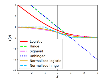
To address the issue of failing to optimize in equation (1), the paper suggests approximately drawing samples from [math]\displaystyle{ \rho_N(x) }[/math] by using co-pseudo-labeling. The methodology is to estimate the expectation over [math]\displaystyle{ \rho_N }[/math]. The authors firstly introduced pseudo-labeling to find the empirical risk in order to solve equation (1) in their setting. However, the over-confidence of the classifier arises from incorrectly predictions of the labels during training. Then the authors proposed co-pseudo-labeling which combined the ideas of pseudo-labeling and co-training, namely Robust IL with Co-pseudo-labeling (RIL-Co). After determining the overall framework of the model, the authors also made a choice of hyper-parameter [math]\displaystyle{ \lambda }[/math]. It is demonstrated that the appropriate value of [math]\displaystyle{ \lambda }[/math]is [math]\displaystyle{ 0.5 \le \lambda \lt 1(x) }[/math]. Specifically, to avoid increasing the impact of pseudo-labels on the risks, the authors decided to use [math]\displaystyle{ \lambda=0.5 }[/math]. In addition, with regard to the choice of symmetric loss, the authors emphasized that any symmetric loss can be used to learn the expert policy with RIL-Co. As Figure 1 shown, the loss can become symmetric after normalization.

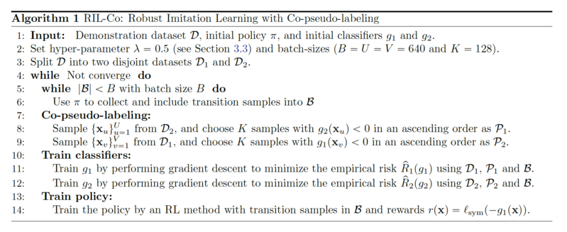
The algorithm of RIC-Co is described with the steps in Figure 2.

Methodology and Results

The RIL-Co model with Average-Precision (AP) loss is benchmarked against other established models: Behavioural Cloning (BC), Forward Inverse Reinforcement Learning (FAIRL), Variational Imitation Learning with Diverse-quality Demonstration (VILD), and three variations of Generative adversarial imitation learning (GAIL) with logistic, unhinged and AP loss functions. All models have the same structure of 2 hidden-layers, with 64 hyperbolic tangent nodes. The policy networks use trust region policy gradient (instead of stochastic gradient like we have seen in our courses), and the classifiers are trained by Adam, with a gradient penalty regularization penalty of 10.

The task supplied to the model to be trained on is to generate a model that walks. There are 4 simulated methods of walking: HalfCheetah, Hopper, Walker2d, and Ant. To generate the demonstrations to train the model on, a regular reinforcement learning model is used with true, known, reward functions. The best performing policy snapshot is then used to generate 10,000 “expert” state-action samples, and the 5 other policy snapshots are used to collect 10,000 “non-expert” state-action samples. The two sets of state-action samples are then mixed with varying noise rates of 0, 0.1, 0.2, 0.3 and 0.4 (e.g., the dataset consisting of 10,000 expert samples and 7500 non-expert samples corresponds to a noise rate of 0.4).

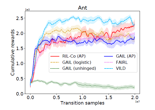
The models are judged on their effectiveness by the cumulative reward. In the experimentation, they observed that RIL-Co performed better than the rest in high noise scenarios (noise rate of 0.2, 0.3 and 0.4), while in low noise scenarios, RIL-Co performs comparably to the best performing alternative. GAIL with AP loss performs better than RIL-Co in low noise scenarios. The authors conject that this is due to co-pseudo-labelling adding additional bias. They propose a fix by varying the hyperparameter lambda from 0, which is equivalent to performing GAIL, to 0.5 as learning progresses.

VILD performs poorly with even small amounts of noisy data (with rate 0.1). The authors believe because VILD has a strict Gaussian noise assumption, and the data is not generated with any noise assumptions, VILD could not accurately estimate the noise distribution and thus performs poorly. BC also performs poorly, which is as expected as BC assumes the demonstrations fed into the model are expert models. The authors also observe that RIL-Co uses fewer transition samples, and thus learns quicker, than other methods in this test. Thus RIL-Co is more data efficient, which is a useful property for a model to have.

An ablation study was conducted, where parts of the model is changed out (such as the loss function) to observe how the model behaves under this change. The loss function was swapped out for a logistic loss to get a better picture of how important a symmetric loss function is to the model. The results indicate that the original AP loss function outperformed the logistic loss, which indicates that using the symmetric loss is important for the model’s ability to be robust.

Another aspect that was tested was the type of noise presented to the model. The RIL-Co model with AP loss was presented with a noisy dataset generated with Gaussian noise. As expected VILD performed much better, since this fits in with the strict Gaussian noise assumption made in the model. RIL-Co achieved performance comparable to VILD given enough transitions, despite no assumption being made in the formulation of the model. This shows promise that RIL-Co performs well under different noise distributions.

Conclusion

A new method for IL from noisy demonstrations is presented, which is more robust than other established methods. Further investigation can be done to see how well this model works under non-simulated data.