Functional regularisation for continual learning with gaussian processes
Presented by
Meixi Chen
Introduction
Continual Learning (CL) refers to the problem where different tasks are fed to a model sequentially, such as training a natural language processing model on different languages over time. A major challenge in CL is a model forgets how to solve earlier tasks. This paper proposed a new framework to regularise Continual Learning (CL) so that it does not forget previously learned tasks. This method, referred to as functional regularisation for Continual Learning, leverages the Gaussian process to construct an approximate posterior belief over the underlying task-specific function. The posterior belief is then used in optimisation as a regulariser to prevent the model from completely deviating from the earlier tasks. The estimation of the posterior functions is carried out under the framework of approximate Bayesian inference.
Previous Work
There are two types of methods that have been widely used in Continual Learning.
Replay/Rehearsal Methods
This type of method stores the data or its compressed form from earlier tasks. The stored data is replayed when learning a new task to mitigate forgetting. It can be used for constraining the optimisation of new tasks or joint training of both previous and current tasks. However, it has two disadvantages: 1) Deciding which data to store often remains heuristic; 2) It requires a large quantity of stored data to achieve good performance.
Regularisation-based Methods
These methods leverage sequential Bayesian inference by putting a prior distribution over the model parameters in the hope to regularise the learning of new tasks. Elastic Weight Consolidation (EWC) and Variational Continual Learning (VCL) are two important methods, both of which make model parameters adaptive to new tasks while regularising weights by prior knowledge from the earlier tasks. Nonetheless, this might still result in an increased forgetting of earlier tasks with long sequences of tasks.
Comparison between the Proposed Method and Previous Methods
Comparison to replay/rehearsal methods
Similarity: It also stores data from earlier tasks.
Difference: Instead of storing a subset of data, it stores a set of inducing points, which can be optimised using criteria from GP literature [2] [3] [4].
Comparison to regularisation-based methods
Similarity: It is also based on approximate Bayesian inference by using a prior distribution that regularises the model updates.
Difference: It constrains the neural network on the space of functions rather than weights by making use of Gaussian processes (GP).
Recap of the Gaussian Process
Definition: A Gaussian process (GP) is a collection of random variables, any finite number of which have a joint Gaussian distribution [1].
The Gaussian process is a non-parametric approach as it can be viewed as an infinite-dimensional generalisation of multivariate normal distributions. In a very informal sense, it can be thought of as a distribution of continuous functions - this is why we make use of GP to perform optimisation in the function space. A Gaussian process over a prediction function [math]\displaystyle{ f(\boldsymbol{x}) }[/math] can be completely specified by its mean function and covariance function (or kernel function), \[\text{Gaussian process: } f(\boldsymbol{x}) \sim \mathcal{GP}(m(\boldsymbol{x}),K(\boldsymbol{x},\boldsymbol{x}'))\] Note that in practice the mean function is typically taken to be 0 because we can always write [math]\displaystyle{ f(\boldsymbol{x})=m(\boldsymbol{x}) + g(\boldsymbol{x}) }[/math] where [math]\displaystyle{ g(\boldsymbol{x}) }[/math] follows a GP with 0 mean. Hence, the GP is characterised by its kernel function.
In fact, we can connect a GP to a multivariate normal (MVN) distribution with 0 mean, which is given by \[\text{Multivariate normal distribution: } \boldsymbol{y} \sim \mathcal{N}(\boldsymbol{0}, \boldsymbol{\Sigma}).\] When we only observe finitely many [math]\displaystyle{ \boldsymbol{x} }[/math], the function's value at these input points is a multivariate normal distribution with covariance matrix parametrised by the kernel function.
Note: Throughout this summary, [math]\displaystyle{ \mathcal{GP} }[/math] refers the the distribution of functions, and [math]\displaystyle{ \mathcal{N} }[/math] refers to the distribution of finite random variables.
A One-dimensional Example of the Gaussian Process
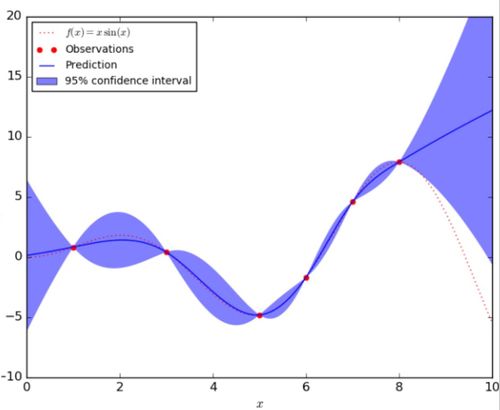
In the figure below, the red dashed line represents the underlying true function [math]\displaystyle{ f(x) }[/math] and the red dots are the observation taken from this function. The blue solid line indicates the predicted function [math]\displaystyle{ \hat{f}(x) }[/math] given the observations, and the blue shaded area corresponds to the uncertainty of the prediction.
A large class of examples of Gaussian processes
The prima facie example of a Gaussian process in continuous time is a Brownian motion. It turns out that Brownian motion is a key ingredient in constructing a large class of Gaussian processes, which can be achieved through the Wiener integral. We write this down as a Proposition and prove it below.
Proposition Let [math]\displaystyle{ B = \{ B_t \}_{t \geq 0} }[/math] be a Brownian motion on a filtered probability space and [math]\displaystyle{ f }[/math] a square integrable deterministic function. Then the process [math]\displaystyle{ X_t }[/math] given by the Wiener integral [math]\displaystyle{ X_t = \int_0^t f(s) dB_s }[/math] is a Gaussian process.
For a reference to several elementary constructions of the Wiener integral, we refer the reader to the textbook by Kuo [6]. Intuitively, the stochastic process [math]\displaystyle{ X_t }[/math] can be thought as the gain or loss of the strategy [math]\displaystyle{ f(s) }[/math] when playing a fair game induced by tracking a Brownian motion.
Proof The Wiener integral of a simple function is the sum of independent centred normal random variables, which is in turn a centred Gaussian process. Since the space of Gaussian processes is closed in [math]\displaystyle{ L^2 (\Omega \times [0,T]) }[/math], as we take the limit as in the construction of the Wiener integral, the process converges and remains a centred Gaussian process. QED
Using the above proposition, one simple example of a Gaussian process is a Brownian bridge, defined as [math]\displaystyle{ Y_t = (1-t) \int_0^t \frac{dB_s}{1-s} }[/math] for [math]\displaystyle{ 0 \leq t \lt 1 }[/math]. This process can be proved to be Gaussian using the proposition proved above.
Methods
Consider a deep neural network in which the final hidden layer provides the feature vector [math]\displaystyle{ \phi(x;\theta)\in \mathbb{R}^K }[/math], where [math]\displaystyle{ x }[/math] is the input data and [math]\displaystyle{ \theta }[/math] are the task-shared model parameters. Importantly, let's assume the task boundaries are known. That is, we know when the input data is switched to a new task. Taking the NLP model as an example, this is equivalent to assuming we know whether each batch of data belongs to English, French, or German dataset. This assumption is important because it allows us to know when to update the task-shared parameter [math]\displaystyle{ \theta }[/math]. The authors also discussed how to detect task boundaries when they are not given, which will be presented later in this summary.
For each specific task [math]\displaystyle{ i }[/math], an output layer is constructed as [math]\displaystyle{ f_i(x;w_i) = w_i^T\phi(x;\theta) }[/math], where [math]\displaystyle{ w_i }[/math] is the task-specific weight. By assuming that the weight [math]\displaystyle{ w_i }[/math] follows a normal distribution [math]\displaystyle{ w_i\sim \mathcal{N}(0, \sigma_w^2I) }[/math], we obtain a distribution over functions: \[f_i(x) \sim \mathcal{GP}(0, k(x,x')), \] where [math]\displaystyle{ k(x,x') = \sigma_w^2 \phi(x;\theta)^T\phi(x';\theta) }[/math]. We can express our posterior belief over [math]\displaystyle{ f_i(x) }[/math] instead of [math]\displaystyle{ w_i }[/math]. Namely, we are interested in estimating
\[\boldsymbol{f}_i|\text{Data} \sim p(\boldsymbol{f}_i|\boldsymbol{y}_i, X_i),\] where [math]\displaystyle{ X_i = \{x_{i,j}\}_{j=1}^{N_i} }[/math] are input vectors and [math]\displaystyle{ \boldsymbol{y}_i = \{y_{i,j}\}_{j=1}^{N_i} }[/math] are output targets so that each [math]\displaystyle{ y_{i,j} }[/math] is assigned to the input [math]\displaystyle{ x_{i,j} \in R^D }[/math]. However, in practice the following approxiation is used:
\[\boldsymbol{f}_i|\text{Data} \overset{approx.}{\sim} \mathcal{N}(\boldsymbol{f}_i|\mu_i, \Sigma_i),\] Instead of having fixed model weight [math]\displaystyle{ w_i }[/math], we now have a distribution for it, which depends on the input data. Then we can summarise information acquired from a task by the estimated distribution of the weights, or equivalently, the distribution of the output functions that depend on the weights. However, we are facing the computational challenge of storing [math]\displaystyle{ \mathcal{O}(N_i^2) }[/math] parameters and keeping in memory the full set of input vector [math]\displaystyle{ X_i }[/math]. To see this, note that the [math]\displaystyle{ \Sigma_i }[/math] is a [math]\displaystyle{ N_i \times N_i }[/math] matrix. Hence, the authors tackle this problem by using the Sparse Gaussian process with inducing points, which is introduced as follows.
Inducing Points: [math]\displaystyle{ Z_i = \{z_{i,j}\}_{j=1}^{M_i} }[/math], which can be a subset of [math]\displaystyle{ X_i }[/math] (the [math]\displaystyle{ i }[/math]-th training inputs) or points lying between the training inputs.
Auxiliary function: [math]\displaystyle{ \boldsymbol{u}_i }[/math], where [math]\displaystyle{ u_{i,j} = f(z_{i,j}) }[/math].
We typically choose the number of inducing points to be a lot smaller than the number of training data. The idea behind the inducing point method is to replace [math]\displaystyle{ \boldsymbol{f}_i }[/math] by the auxiliary function [math]\displaystyle{ \boldsymbol{u}_i }[/math] evaluated at the inducing inputs [math]\displaystyle{ Z_i }[/math]. Intuitively, we are also assuming the inducing inputs [math]\displaystyle{ Z_i }[/math] contain enough information to make inference about the "true" [math]\displaystyle{ \boldsymbol{f}_i }[/math], so we can replace [math]\displaystyle{ X_i }[/math] by [math]\displaystyle{ Z_i }[/math].
Now we can introduce how to learn the first task when no previous knowledge has been acquired.
Learning the First Task
In learning the first task, the goal is to generate the first posterior belief given this task: [math]\displaystyle{ p(\boldsymbol{u}_1|\text{Data}) }[/math]. We learn this distribution by approximating it by a variational distribution: [math]\displaystyle{ q(\boldsymbol{u}_1) }[/math]. That is, [math]\displaystyle{ p(\boldsymbol{u}_1|\text{Data}) \approx q(\boldsymbol{u}_1) }[/math]. We can parametrise [math]\displaystyle{ q(\boldsymbol{u}_1) }[/math] as [math]\displaystyle{ \mathcal{N}(\boldsymbol{u}_1 | \mu_{u_1}, L_{u_1}L_{u_1}^T) }[/math], where [math]\displaystyle{ L_{u_1} }[/math] is the lower triangular Cholesky factor. I.e., [math]\displaystyle{ \Sigma_{u_1}=L_{u_1}L_{u_1}^T }[/math]. Next, we introduce how to estimate [math]\displaystyle{ q(\boldsymbol{u}_1) }[/math], or equivalently, [math]\displaystyle{ \mu_{u_1} }[/math] and [math]\displaystyle{ L_{u_1} }[/math], using variational inference.
Given the first task with data [math]\displaystyle{ (X_1, \boldsymbol{y}_1) }[/math], we can use a variational distribution [math]\displaystyle{ q(\boldsymbol{f}_1, \boldsymbol{u}_1) }[/math] that approximates the exact posterior distribution [math]\displaystyle{ p(\boldsymbol{f}_1, \boldsymbol{u}_1| \boldsymbol{y}_1) }[/math], where \[q(\boldsymbol{f}_1, \boldsymbol{u}_1) = p_\theta(\boldsymbol{f}_1|\boldsymbol{u}_1)q(\boldsymbol{u}_1)\] \[p(\boldsymbol{f}_1, \boldsymbol{u}_1| \boldsymbol{y}_1) = p_\theta(\boldsymbol{f}_1|\boldsymbol{u}_1, \boldsymbol{y}_1)p_\theta(\boldsymbol{u}_1|\boldsymbol{y}_1).\] Note that we use [math]\displaystyle{ p_\theta(\cdot) }[/math] to denote the Gaussian distribution form with kernel parametrised by a common [math]\displaystyle{ \theta }[/math].
Hence, we can jointly learn [math]\displaystyle{ q(\boldsymbol{u}_1) }[/math] and [math]\displaystyle{ \theta }[/math] by minimising the KL divergence \[\text{KL}(p_{\theta}(\boldsymbol{f}_1|\boldsymbol{u}_1)q(\boldsymbol{u}_1) \ || \ p_{\theta}(\boldsymbol{f}_1|\boldsymbol{u}_1, \boldsymbol{y}_1)p_{\theta}(\boldsymbol{u}_1|\boldsymbol{y}_1)),\] which is equivalent to maximising the Evidence Lower Bound (ELBO) \[\mathcal{F}({\theta}, q(\boldsymbol{u}_1)) = \sum_{j=1}^{N_1} \mathbb{E}_{q(f_1, j)}[\log p(y_{1,j}|f_{1,j})]-\text{KL}(q(\boldsymbol{u}_1) \ || \ p_{\theta}(\boldsymbol{u}_1)).\]
Learning the Subsequent Tasks
After learning the first task, we only keep the inducing points [math]\displaystyle{ Z_1 }[/math] and the parameters of [math]\displaystyle{ q(\boldsymbol{u}_1) }[/math], both of which act as a task summary of the first task. Note that [math]\displaystyle{ \theta }[/math] also has been updated based on the first task. In learning the [math]\displaystyle{ k }[/math]-th task, we can use the posterior belief [math]\displaystyle{ q(\boldsymbol{u}_1), q(\boldsymbol{u}_2), \ldots, q(\boldsymbol{u}_{k-1}) }[/math] obtained from the preceding tasks to regularise the learning, and produce a new task summary [math]\displaystyle{ (Z_k, q(\boldsymbol{u}_k)) }[/math]. Similar to the first task, now the objective function to be maximised is \[\mathcal{F}(\theta, q(\boldsymbol{u}_k)) = \underbrace{\sum_{j=1}^{N_k} \mathbb{E}_{q(f_k, j)}[\log p(y_{k,j}|f_{k,j})]- \text{KL}(q(\boldsymbol{u}_k) \ || \ p_{\theta}(\boldsymbol{u}_k))}_{\text{objective for the current task}} - \underbrace{\sum_{i=1}^{k-1}\text{KL}(q(\boldsymbol{u}_i) \ || \ p_{\theta}(\boldsymbol{u}_i)))}_{\text{regularisation from previous tasks}}\]
As a result, we regularise the learning of a new task by the sum of KL divergence terms [math]\displaystyle{ \sum_{i=1}^{k-1}\text{KL}(q(\boldsymbol{u}_i) \ || \ p_\theta(\boldsymbol{u}_i)) }[/math], where each [math]\displaystyle{ q(\boldsymbol{u}_i) }[/math] encodes the knowledge about an earlier task [math]\displaystyle{ i \lt k }[/math]. To make the optimisation computationally efficient, we can sub-sample the KL terms in the sum and perform stochastic approximation over the regularisation term.
Alternative Inference for the Current Task
Given this framework of sparse GP inference, the author proposed a further improvement to obtain more accurate estimates of the posterior belief [math]\displaystyle{ q(\boldsymbol{u}_k) }[/math]. That is, performing inference over the current task in the weight space. Due to the trade-off between accuracy and scalability imposed by the number of inducing points, we can use a full Gaussian viariational approximation \[q(w_k) = \mathcal{N}(w_k|\mu_{w_k}, \Sigma_{w_k})\] by letting [math]\displaystyle{ f_k(x; w_k) = w_k^T \phi(x; \theta) }[/math], [math]\displaystyle{ w_k \sim \mathcal{N}(0, \sigma_w^2 I) }[/math]. The objective becomes \[\mathcal{F}(\theta, q(w_k)) = \underbrace{\sum_{j=1}^{N_k} \mathbb{E}_{q(f_k, j)}[\log p(y_{k,j}|w_k^T \phi(x_{k,j}; \theta))]- \text{KL}(q(w_k) \ || \ p(w_k))}_{\text{objective for the current task}} - \underbrace{\sum_{i=1}^{k-1}\text{KL}(q(\boldsymbol{u}_i) \ || \ p_{\theta}(\boldsymbol{u}_i)))}_{\text{regularisation from previous tasks}}\]
After learning [math]\displaystyle{ \mu_{w_k} }[/math] and [math]\displaystyle{ \Sigma_{w_k} }[/math], we can also compute the posterior distribution over their function values [math]\displaystyle{ \boldsymbol{u}_k }[/math] according to [math]\displaystyle{ q(\boldsymbol{u}_k) = \mathcal{N}(\boldsymbol{u}_k|\mu_{u_k}, L_{u_k}L_{u_k}^T }[/math]), where [math]\displaystyle{ \mu_{u_k} = \Phi_{Z_k}\mu_{w_k} }[/math], [math]\displaystyle{ L_{u_k}=\Phi_{Z_k}L_{w_k} }[/math], and [math]\displaystyle{ \Phi_{Z_k} }[/math] stores as rows the feature vectors evaluated at [math]\displaystyle{ Z_k }[/math].
The figure below is a depiction of the proposed method.
Selection of the Inducing Points
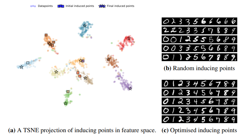
In practice, a simple but effective way to select inducing points is to select a random set [math]\displaystyle{ Z_k }[/math] of the training inputs [math]\displaystyle{ X_k }[/math]. In this paper, the authors proposed a structured way to select them. The proposed method is an unsupervised criterion that only depends on the training inputs, which quantifies how well the full kernel matrix [math]\displaystyle{ K_{X_k} }[/math] can be constructed from the inducing inputs. This is done by minimizing the trace of the covariance matrix of the prior GP conditional [math]\displaystyle{ p(\boldsymbol{f}_k|\boldsymbol{u}_k) }[/math]: \[\mathcal{T}(Z_k)=\text{tr}(K_{X_k} - K_{X_kZ_K}K_{Z_k}^{-1}K_{Z_kX_k}),\] where [math]\displaystyle{ K_{X_k} = K(X_k, X_k), K_{X_kZ_K} = K(X_k, Z_k), K_{Z_k} = K(Z_k, Z_k) }[/math], and [math]\displaystyle{ K(\cdot, \cdot) }[/math] is the kernel function parametrised by [math]\displaystyle{ \theta }[/math]. This method promotes finding inducing points [math]\displaystyle{ Z_k }[/math] that are spread evenly in the input space. As an example, see the following figure where the final selected inducing points are spread out in different clusters of data. On the right side of the image, the round dots represent the data points and each colour corresponds to a different label. The left part of the image shows how optimised inducing images cover examples from all classes as opposed to the randomised inducing points where each example could have a skewed number of points from the same class.
Prediction
Given a test data point [math]\displaystyle{ x_{i,*} }[/math], we can obtain the predictive density function of its output [math]\displaystyle{ y_{i,*} }[/math] given by \begin{align*} p(y_{i,*}) &= \int p(y_{i,*}|f_{i,*}) p_\theta(f_{i,*}|\boldsymbol{u}_i)q(\boldsymbol{u}_i) d\boldsymbol{u}_i df_{i,*}\\ &= \int p(y_{i,*}|f_{i,*}) q_\theta(f_{i,*}) df_{i,*}, \end{align*} where [math]\displaystyle{ q_\theta(f_{i,*})=\mathcal{N}(f_{i,*}| \mu_{i,*}, \sigma_{i,*}^2) }[/math] with known mean and variance \begin{align*} \mu_{i,*} &= \mu_{u_i}^TK_{Z_i}^{-1} k_{Z_kx_i,*}\\ \sigma_{i,*}^2 &= k(x_{i,*}, x_{i,*}) + k_{Z_ix_i,*}^T K_{Z_i}^{-1}[L_{u_i}L_{u_i}^T - K_{Z_i}] K_{Z_i}^{-1} k_{Z_ix_i,*} \end{align*} Note that all the terms in [math]\displaystyle{ \mu_{i,*} }[/math] and [math]\displaystyle{ \sigma_{i,*}^2 }[/math] are either already estimated or depend on some estimated parameters.
It is important to emphasise that the mean [math]\displaystyle{ \mu_{i,*} }[/math] can be further rewritten as [math]\displaystyle{ \mu_{u_i}^TK_{Z_i}^{-1}\Phi_{Z_i}\phi(x_{i,*};\theta) }[/math], which, notably, depends on [math]\displaystyle{ \theta }[/math]. This means that the expectation of [math]\displaystyle{ f_{i,*} }[/math] changes over time as more tasks are learned, so the overall prediction will not be out of date. In comparison, if we use a distribution of weights [math]\displaystyle{ w_i }[/math], the mean of the distribution will remain unchanged over time, thus resulting in obsolete prediction.
Detecting Task Boundaries
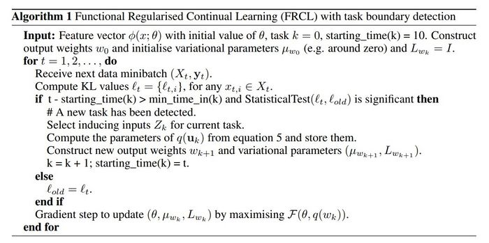
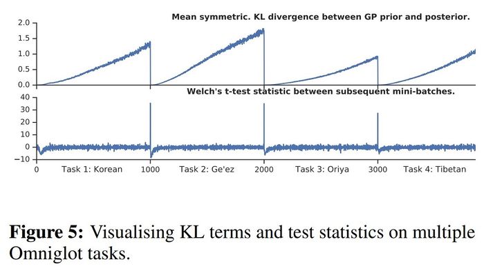
In the previous discussion, we have assumed the task boundaries are known, but this assumption is often unrealistic in the practical setting. Therefore, the authors introduced a way to detect task boundaries using GP predictive uncertainty. This is done by measuring the distance between the GP posterior density of a new task data and the prior GP density using symmetric KL divergence. We can measure the distance between the GP posterior density of a new task data and the prior GP density using symmetric KL divergence. We denote this score by [math]\displaystyle{ \ell_i }[/math], which can be interpreted as a degree of surprise about [math]\displaystyle{ x_i }[/math] - the smaller is [math]\displaystyle{ \ell_i }[/math] the more surprising is [math]\displaystyle{ x_i }[/math]. Before making any updates to the parameter, we can perform a statistical test between the values [math]\displaystyle{ \{\ell_i\}_{i=1}^b }[/math] for the current batch and those from the previous batch [math]\displaystyle{ \{\ell_i^{old}\}_{i=1}^b }[/math]. A natural choice is Welch's t-test, which is commonly used to compare two groups of data with unequal variance.
The figure below illustrates the intuition behind this method. With red dots indicating a new task, we can see the GP posterior (green line) reverts back to the prior (purple line) when it encounters the new task. Hence, this explains why a small [math]\displaystyle{ \ell_i }[/math] corresponds to a task switch.
Algorithm
Experiments
The authors aimed to answer three questions:
- How does FRCL compare to state-of-the-art algorithms for Continual Learning?
- How does the criterion for inducing point selection affect accuracy?
- When ground truth task boundaries are not given, does the detection method mentioned above succeed in detecting task changes?
Comparison to state-of-the-art algorithms
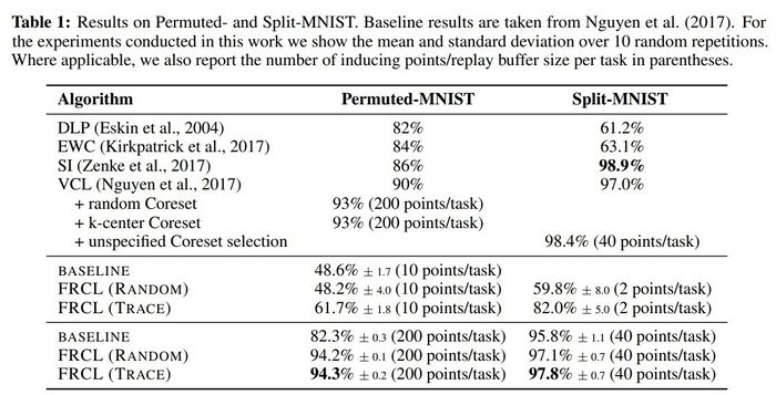
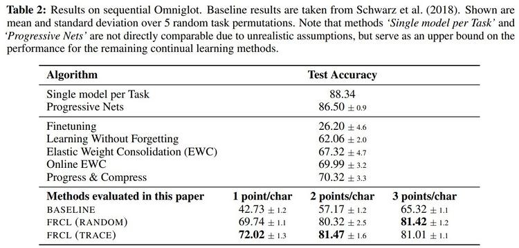
The proposed method was applied to two MNIST-variation datasets (in Table 1) and the more challenging Omniglot benchmark (in Table 2). They compared the method with randomly selected inducing points, denoted by FRCL(RANDOM), and the method with inducing points optimised using trace criterion, denoted by FRCL(TRACE). The baseline method corresponds to a simple replay-buffer method described in the appendix of the paper. Both tables show that the proposed method gives strong results, setting a new state-of-the-art result on both Permuted-MNIST and Omniglot.
Comparison of different criteria for inducing points selection
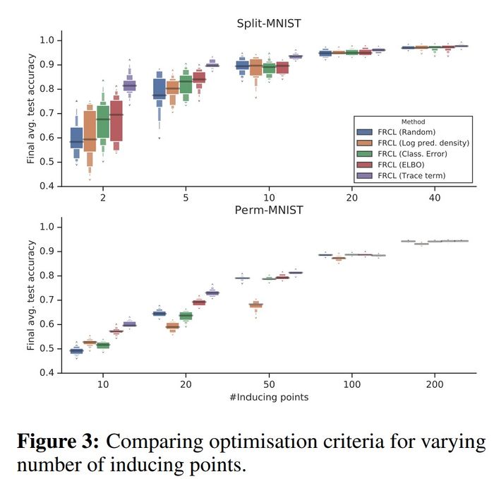
As can be seen from the figure below, the purple box corresponding to FRCL(TRACE) is consistently higher than the others, and in particular, this difference is larger when the number of inducing points is smaller. Hence, a structured selection criterion becomes more and more important when the number of inducing points reduces.
Efficacy in detecting task boundaries
From the following figure, we can observe that both the mean symmetric KL divergence and the t-test statistic always drop when a new task is introduced. Hence, the proposed method for detecting task boundaries indeed works.
Conclusions
The proposed method unifies both the regularisation-based method and the replay/rehearsal method in Continual Learning. It was able to overcome the disadvantages of both methods. Moreover, the Bayesian framework allows a probabilistic interpretation of deep neural networks. From the experiments we can make the following conclusions:
- The proposed method sets new state-of-the-art results on Permuted-MNIST and Omniglot, and is comparable to the existing results on Split-MNIST.
- A structured criterion for selecting inducing points becomes increasingly important with a decreasing number of inducing points.
- The method is able to detect task boundary changes when they are not given.
Future work can include enforcing a fixed memory buffer where the summary of all previously seen tasks is compressed into one summary. It would also be interesting to investigate the application of the proposed method to other domains such as reinforcement learning.
Critiques
This paper presents a new way for remembering previous tasks by reducing the KL divergence of variational distribution: [math]\displaystyle{ q(\boldsymbol{u}_1) }[/math] and [math]\displaystyle{ p_\theta(u_1) }[/math]. The ideas in the paper are interesting and experiments support the effectiveness of this approach. After reading the summary, some points came to my mind as follows:
The main problem with Gaussian Process is its test-time computational load where a Gaussian Process needs a data matrix and a kernel for each prediction. Although this seems to be natural as Gaussian Process is non-parametric and except for data, it has no source of knowledge, however, this comes with computational and memory costs which makes this difficult to employ them in practice. In this paper, the authors propose to employ a subset of training data namely "Inducing Points" to mitigate these challenges. They proposed to choose Inducing Points either at random or based on an optimisation scheme where Inducing Points should approximate the kernel. Although in the paper authors formulate the problem of Inducing Points in their formulation setting, this is not a new approach in the field and previously known as the Finding Exemplars problem. In fact, their formulation is very similar to the ideas in the following paper:
Elhamifar, Ehsan, Guillermo Sapiro, and Rene Vidal. Finding exemplars from pairwise dissimilarities via simultaneous sparse recovery. Advances in Neural Information Processing Systems. 2012.
More precisely the main is difference is that in the current paper kernel matrix and in the mentioned paper dissimilarities are employed to find Exemplars or induced points.
Moreover, one unanswered question is how to determine the number of examplers as they play an important role in this algorithm.
Besides, one practical point is replacing the covariance matrix with its Cholesky decomposition. In practice covariance matrices are positive semi-definite in general while to the best of my knowledge Cholesky decomposition can be used for positive definite matrices. Considering this, I am not sure what happens if the Cholesky decomposition is explicitly applied to the covariance matrix.
Finally, the number of regularisation terms [math]\displaystyle{ \sum_{i=1}^{k-1}\text{KL}(q(\boldsymbol{u}_i) \ || \ p_\theta(\boldsymbol{u}_i)) }[/math] growth linearly with number of tasks, I am not sure how this algorithm works when number of tasks increases. Clearly, apart from computational cost, having many regularisation terms can make optimisation more difficult.
The provided experiments seem interesting and quite enough and did a good job highlighting different facets of the paper but it would be better if these two additional results can be provided as well: (1) How well-calibrated are FRCL-based classifiers? (2) How impactful is the hybrid representation for test-time performance?
The problem of balancing short term and long term memory of rewards is an important problem in reinforcement learning. It would be interesting to consider the applications of this algorithm and its variants to reinforcement learning problems. Additionally, for problems where the rewards may change over time, it would be interesting to compare this method to some of the existing ones.
Source Code
https://github.com/AndreevP/FRCL
References
[1] Rasmussen, Carl Edward and Williams, Christopher K. I., 2006, Gaussian Processes for Machine Learning, The MIT Press.
[2] Quinonero-Candela, Joaquin and Rasmussen, Carl Edward, 2005, A Unifying View of Sparse Approximate Gaussian Process Regression, Journal of Machine Learning Research, Volume 6, P1939-1959.
[3] Snelson, Edward and Ghahramani, Zoubin, 2006, Sparse Gaussian Processes using Pseudo-inputs, Advances in Neural Information Processing Systems 18, P1257-1264.
[4] Michalis K. Titsias, Variational Learning of Inducing Variables in Sparse Gaussian Processes, 2009, Proceedings of the 12th International Conference on Artificial Intelligence and Statistics, Volume 5, P567-574.
[5] Michalis K. Titsias, Jonathan Schwarz, Alexander G. de G. Matthews, Razvan Pascanu, Yee Whye Teh, 2020, Functional Regularisation for Continual Learning with Gaussian Processes, ArXiv abs/1901.11356.
[6] Kuo, H. "Introduction to Stochastic Integration Springer." Berlin Heidelberg (2006).


