User:Yktan
Introduction
Much of the success in training deep neural networks (DNNs) is due to the collection of large datasets with human-annotated labels. However, human annotation is both a time-consuming and expensive task, especially for data that requires expertise such as medical data. Furthermore, certain datasets will be noisy due to the biases introduced by different annotators. Data obtained in large quantities through searching for images in search engines and data downloaded from social media sites (in a manner abiding by privacy and copyright laws) are especially noisy, since the labels are generally inferred from tags to save on human-annotation cost.
There are a few existing approaches to use datasets with noisy labels. In learning with noisy labels (LNL), most methods take a loss correction approach. Other LNL methods estimate a noise transition matrix and employ it to correct the loss function. An example of a popular loss correction approach is the bootstrapping loss approach. Another approach to reduce annotation cost is semi-supervised learning (SSL), where the training data consists of labeled and unlabeled samples. The main limitation of these methods is that they do not perform well under high noise ratio and cause overfitting.
This paper introduces DivideMix, which combines approaches from LNL and SSL. One unique thing about DivideMix is that it discards sample labels that are highly likely to be noisy and leverages these noisy samples as unlabeled data instead. This prevents the model from overfitting and improves generalization performance. Key contributions of this work are: 1) Co-divide, which trains two networks simultaneously, aims to improve generalization and avoid confirmation bias. 2) During the SSL phase, an improvement is made on an existing method (MixMatch) by combining it with another method (MixUp). 3) Significant improvements to state-of-the-art results on multiple conditions are experimentally shown while using DivideMix. Extensive ablation study and qualitative results are also shown to examine the effect of different components.
Motivation
While much has been achieved in training DNNs with noisy labels and SSL methods individually, not much progress has been made in exploring their underlying connections and building on top of the two approaches simultaneously.
Existing LNL methods aim to correct the loss function by:
- Treating all samples equally and correcting loss explicitly or implicitly through relabelling of the noisy samples
- Reweighting training samples or separating clean and noisy samples, which results in correction of the loss function
A few examples of LNL methods include:
- Estimating the noise transition matrix, which denotes the probability of clean labels flipping to noisy labels, to correct the loss function
- Leveraging the predictions from DNNs to correct labels and using them to modify the loss
- Reweighting samples so that noisy labels contribute less to the loss
However, these methods all have downsides: it is very challenging to correctly estimate the noise transition matrix in the first method; for the second method, DNNs tend to overfit to datasets with high noise ratio; and for the third method, we need to be able to identify clean samples, which has also proven to be challenging.
On the other hand, SSL methods mostly leverage unlabeled data using regularization to improve model performance. A recently proposed method, MixMatch, incorporates the two classes of regularization. These classes are consistency regularization which enforces the model to produce consistent predictions on augmented input data, and entropy minimization which encourages the model to give high-confidence predictions on unlabeled data, as well as MixUp regularization.
DivideMix partially adopts LNL in that it removes the labels that are highly likely to be noisy by using co-divide to avoid the confirmation bias problem. It then utilizes the noisy samples as unlabeled data and adopts an improved version of MixMatch (an SSL technique) which accounts for the label noise during the label co-refinement and co-guessing phase. By incorporating SSL techniques into LNL and taking the best of both worlds, DivideMix aims to produce highly promising results in training DNNs by better addressing the confirmation bias problem, more accurately distinguishing and utilizing noisy samples, and performing well under high levels of noise.
Model Architecture and Algorithm
DivideMix leverages semi-supervised learning to achieve effective modeling. The sample is first split into a labeled set and an unlabeled set. This is achieved by fitting a Gaussian Mixture Model as a per-sample loss distribution. The unlabeled set is made up of data points with discarded labels deemed noisy.
Then, to avoid confirmation bias, which is typical when a model is self-training, two models are being trained simultaneously to filter error for each other. This is done by dividing the data into clean labeled set (X)and a noisy unlabeled set (U) using one model and then training the other model on the data set U. This algorithm, known as Co-divide, keeps the two networks from converging when training, which avoids the bias from occurring. Gaussian Mixture Model is better at distinguishing X and U, whereas Beta Mixture Model produces flat distribution and fails to label correctly. Being diverged also offers the two networks distinct abilities to filter different types of error, making the model more robust to noise. However, the model could still have confirmation error where both model would prone to make and confirm the same mistake. Figure 1 describes the algorithm in graphical form.

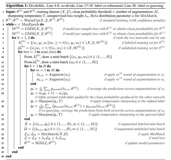
For each epoch, the network divides the dataset into a labeled set consisting of clean data, and an unlabeled set consisting of noisy data, which is then used as training data for the other network, where training is done in mini-batches. For each batch of the labelled samples, co-refinement is performed by using the ground truth label [math]\displaystyle{ y_b }[/math], the predicted label [math]\displaystyle{ p_b }[/math], and the posterior is used as the weight, [math]\displaystyle{ w_b }[/math].
Then, a sharpening function is implemented on this weighted sum to produce the estimate with reduced temperature, [math]\displaystyle{ \hat{y}_b }[/math].
Using all these predicted labels, the unlabeled samples will then be assigned a "co-guessed" label, which should produce a more accurate prediction. Having calculated all these labels, MixMatch is applied to the combined mini-batch of labeled, [math]\displaystyle{ \hat{X} }[/math] and unlabeled data, [math]\displaystyle{ \hat{U} }[/math], where, for a pair of samples and their labels, one new sample and new label is produced. More specifically, for a pair of samples [math]\displaystyle{ (x_1,x_2) }[/math] and their labels [math]\displaystyle{ (p_1,p_2) }[/math], the mixed sample [math]\displaystyle{ (x',p') }[/math] is:
[math]\displaystyle{ \begin{alignat}{2} \lambda &\sim Beta(\alpha, \alpha) \\ \lambda ' &= max(\lambda, 1 - \lambda) \\ x' &= \lambda ' x_1 + (1 - \lambda ' ) x_2 \\ p' &= \lambda ' p_1 + (1 - \lambda ' ) p_2 \\ \end{alignat} }[/math]
MixMatch transforms [math]\displaystyle{ \hat{X} }[/math] and [math]\displaystyle{ \hat{U} }[/math] into [math]\displaystyle{ X' }[/math] and [math]\displaystyle{ U' }[/math]. Then, the loss on [math]\displaystyle{ X' }[/math], [math]\displaystyle{ L_X }[/math] (Cross-entropy loss) and the loss on [math]\displaystyle{ U' }[/math], [math]\displaystyle{ L_U }[/math] (Mean Squared Error) are calculated. A regularization term, [math]\displaystyle{ L_{reg} }[/math], is introduced to regularize the model's average output across all samples in the mini-batch. Then, the total loss is calculated as:
where [math]\displaystyle{ \lambda_r }[/math] is set to 1, and [math]\displaystyle{ \lambda_u }[/math] is used to control the unsupervised loss.
Lastly, the stochastic gradient descent formula is updated with the calculated loss, [math]\displaystyle{ L }[/math], and the estimated parameters, [math]\displaystyle{ \boldsymbol{ \theta } }[/math].
The full algorithm is shown below.

Then, when the model is warmed up, it is trained on all data using standard cross-entropy to initially converge the model, but with a regulatory negative entropy term [math]\displaystyle{ \mathcal{H} = -\sum_{c}\text{p}^\text{c}_\text{model}(x;\theta)\log(\text{p}^\text{c}_\text{model}(x;\theta)) }[/math], where [math]\displaystyle{ \text{p}^\text{c}_\text{model} }[/math] is the softmax output probability for class c. This term penalizes confident predictions during the warm up to prevent overfitting to noise during the warm up, which can happen when there is asymmetric noise.
Results
Applications
The method was validated using four benchmark datasets: CIFAR-10, CIFAR100 (Krizhevsky & Hinton, 2009) which contain 50K training images and 10K test images of size 32 × 32), Clothing1M (Xiao et al., 2015), and WebVision (Li et al., 2017a). Two types of label noise are used in the experiments: symmetric and asymmetric. An 18-layer PreAct Resnet (He et al., 2016) is trained using SGD with a momentum of 0.9, a weight decay of 0.0005, and a batch size of 128. The network is trained for 300 epochs. The initial learning rate was set to 0.02 and reduced by a factor of 10 after 150 epochs. Before applying the Co-divide and MixMatch strategies, the models were first independently trained over the entire dataset using cross-entropy loss during a "warm-up" period. Initially, training the models in this way prepares a more regular distribution of losses to improve upon in subsequent epochs. The warm-up period is 10 epochs for CIFAR-10 and 30 epochs for CIFAR-100. For all CIFAR experiments, we use the same hyperparameters M = 2, T = 0.5, and α = 4. τ is set as 0.5 except for 90% noise ratio when it is set as 0.6.
Comparison of State-of-the-Art Methods
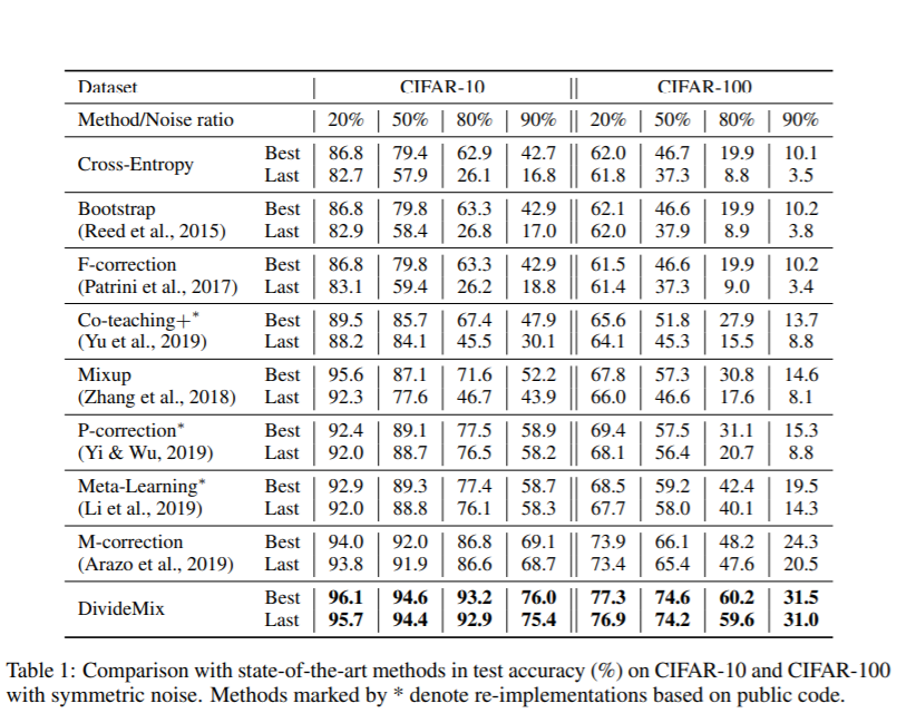
The effectiveness of DivideMix was shown by comparing the test accuracy with the most recent state-of-the-art methods: Meta-Learning (Li et al., 2019) proposes a gradient-based method to find model parameters that are more noise-tolerant; Joint-Optim (Tanaka et al., 2018) and P-correction (Yi & Wu, 2019) jointly optimize the sample labels and the network parameters; M-correction (Arazo et al., 2019) models sample loss with BMM and apply MixUp. The following are the results on CIFAR-10 and CIFAR-100 with different levels of symmetric label noise ranging from 20% to 90%. Both the best test accuracy across all epochs and the averaged test accuracy over the last 10 epochs were recorded in the following table:

From table 1, the author noticed that none of these methods can consistently outperform others across different datasets. M-correction excels at symmetric noise, whereas Meta-Learning performs better for asymmetric noise. DivideMix outperforms state-of-the-art methods by a large margin across all noise ratios. The improvement is substantial (∼10% of accuracy) for the more challenging CIFAR-100 with high noise ratios.
DivideMix was compared with the state-of-the-art methods with the other two datasets: Clothing1M and WebVision. It also shows that DivideMix consistently outperforms state-of-the-art methods across all datasets with different types of label noise. For WebVision, DivideMix achieves more than 12% improvement in top-1 accuracy.
Ablation Study
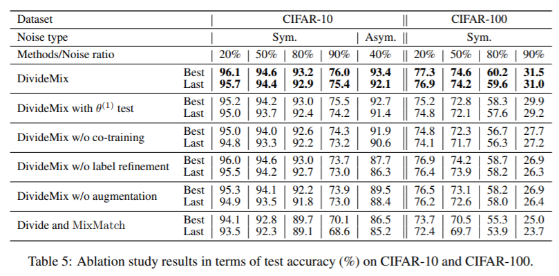
The effect of removing different components to provide insights into what makes DivideMix successful. We analyze the results in Table 5 as follows.

The authors combined self-divide with the original MixMatch as a naive baseline for using SLL in LNL. They also find that both label refinement and input augmentation are beneficial for DivideMix. Label refinement is important for high noise ratio due because samples that are noisier would be incorrectly divided into the labeled set. Augmentation upgrades model performance by creating more reliable predictions and by achieving consistent regularization. In addition, the performance drop was seen in the DivideMix w/o co-training highlights the disadvantage of self-training; the model still has dataset division, label refinement and label guessing, but they are all performed by the same model.
Conclusion
This paper provides a new and effective algorithm for learning with noisy labels by using highly noisy data unlabelled data in a Semi-Supervised Learning framework. The DivideMix method trains two networks simultaneously and utilizes co-guessing and co-labeling effectively, therefore it is a robust approach to deal with noise in datasets. Also, the DivideMix method has been tested using various datasets with the results consistently being one of the best when compared to the state-of-the-art methods through extensive experiments.
Future work of DivideMix is to create an adaptation for other applications such as Natural Language Processing, and incorporating the ideas of SSL and LNL into DivideMix architecture.
Critiques/ Insights
1. While combining both models makes the result better, the author did not show the relative time increase using this new combined methodology, which is very crucial considering training a large amount of data, especially for images. In addition, it seems that the author did not perform much on hyperparameters tuning for the combined model.
2. There is an interesting insight, which is when the noise ratio increases from 80% to 90%, the accuracy of DivideMix drops dramatically in both datasets.
3. There should be a further explanation of why the learning rate drops by a factor of 10 after 150 epochs.
4. It would be interesting to see the effectiveness of this method in other domains such as NLP. I am not aware of noisy training datasets available in NLP, but surely this is an important area to focus on, as much of the available data is collected from noisy sources from the web.
5. The paper implicitly assumes that a Gaussian mixture model (GMM) is sufficiently capable of identifying noise. Given the nature of a GMM, it would work well for noise that is distributed by a Gaussian distribution but for all other noise, it would probably be only asymptotic. The paper should present theoretical results on the noise that are Exponential, Rayleigh, etc. This is particularly important because the experiments were done on massive datasets, but they do not directly address the case when there are not many data points.
6. Comparing the training result on these benchmark datasets makes the algorithm quite comprehensive. This is a very insightful idea to maintain two networks to avoid bias from occurring.
7. The current benchmark accuracy for CIFAR-10 is 99.7, CIFAR-100 is 96.08 using EffNet-L2 in 2020. In 2019, CIFAR-10 is 99.37, CIFAR-100 is 93.51 using BiT-L.(based on paperswithcode.com) As there exists better methods, it would be nice to know why the authors chose these state-of-the-art methods to compare the test accuracy.
8. Another interesting observation is that DivideMix seems to maintain a similar accuracy while some methods give unstable results. That shows the reliability of the proposed algorithm.
9. It would be interesting to see if the drop in accuracy from increasing the noise ratio to 90% is a result of a low porportion or low number of clean labels. That is, would increasing the size of the training set but keeping the noise ratio at 90% result in increased accuracy?
10. For Ablation Study part, the paper also introduced a study on the Robustness of Testing Marking Methods Noise, including AUC for classification of clean/noisy samples of CIFAR-10 training data. And it shows that the method can effectively separate clean and noisy samples as training proceeds.
11. It is interesting how unlike common methods, the method in this paper discards the labels that are highly likely to be noisy. It also utilizes the noisy samples as unlabeled data to regularize training in a SSL manner. This model can better distinguish and utilize noisy samples.
12. In the result section, the author gives us a comprehensive understanding of this algorithm by introducing the applications and the comparison of it with respect to similar methods. It would be attractive if in the application part, the author could indicate how the application relative to our daily life.
13. High quality data is very important for training Machine learning systems. Preparing the data to train ML systems requires data annotations which are prone to errors and are time-consuming. It is interesting to note how paper 14 and this paper aims to approach this problem from different perspectives. Paper 14 introduces CSL algorithm that learns from confused or Noisy data to find the tasks associated with them. And this paper proposes an algorithm that shows good performance when learning from noisy data. Hence both the papers seem to tackle similar problem and implementing the approaches described in both the papers when handling noisy data can be twice helpful.
14. Noise exists in all big data, and big data is what we are dealing with in real life nowadays. Having an effective noise eliminating method such as Dividemix is important to us.
15. The DivideMix consistently outperforms state-of-the-art methods across the given datasets, but how about some other potential datasets? If it can be given that it has advantages for a certain type of potential dataset, it will be a better discussion.
16. It would be better if there was more information regarding four benchmark datasets (CIFAR-10, CIFAR100, Clothing1M, and WebVision) so that readers could be aware of the properties or differences of those datasets.
17. It would be interesting to compare the computational cost of this model versus others. Would it be more computationally faster to use in real world applications?
References
[1] Eric Arazo, Diego Ortego, Paul Albert, Noel E. O’Connor, and Kevin McGuinness. Unsupervised label noise modeling and loss correction. In ICML, pp. 312–321, 2019.
[2] David Berthelot, Nicholas Carlini, Ian J. Goodfellow, Nicolas Papernot, Avital Oliver, and Colin Raffel. Mixmatch: A holistic approach to semi-supervised learning. NeurIPS, 2019.
[3] Yifan Ding, Liqiang Wang, Deliang Fan, and Boqing Gong. A semi-supervised two-stage approach to learning from noisy labels. In WACV, pp. 1215–1224, 2018.