IPBoost
Presented by
Casey De Vera, Solaiman Jawad
Introduction
Boosting is an important and a fairly standard technique in a classification that combines several base learners (learners which have a “low accuracy”), into one boosted learner (learner with a “high accuracy”). Pioneered by the AdaBoost approach of Freund & Schapire, in recent decades there has been extensive work on boosting procedures and analyses of their limitations.
In a nutshell, boosting procedures are (typically) iterative schemes that roughly work as follows:
Let [math]\displaystyle{ T }[/math] represents the number of iteration and [math]\displaystyle{ t }[/math] represents the iterator.
for [math]\displaystyle{ t= 1, \cdots, T }[/math] do the following:
- 1. Train a learner [math]\displaystyle{ \mu_t }[/math] from a given class of base learners on the data distribution [math]\displaystyle{ \mathcal D_t }[/math]
- 2. Evaluate the performance of [math]\displaystyle{ \mu_t }[/math] by computing its loss.
- 3. Push weight of the data distribution [math]\displaystyle{ \mathcal D_t }[/math] towards the misclassified examples leading to [math]\displaystyle{ \mathcal D_{t+1} }[/math], usually a relatively good model will have a higher weight on those data that misclassified.
Finally, the learners are combined with some form of voting (e.g., soft or hard voting, averaging, thresholding).

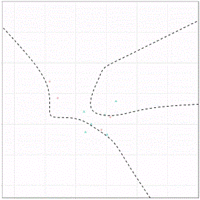
A close inspection of most boosting procedures reveals that they solve an underlying convex optimization problem over a convex loss function using coordinate gradient descent. Boosting schemes of this type are often referred to as convex potential boosters. These procedures can achieve exceptional performance on many data sets if the data is correctly labeled. However, they can be trounced by a small number of incorrect labels, which can be quite challenging to fix. We try to solve misclassified examples by moving the weights around, which results in bad performance on unseen data (Shown by zoomed example to the right). In fact, in theory, providing the class of base learners is rich enough, a perfect strong learner can be constructed with accuracy 1; however, clearly, such a learner might not necessarily generalize well. Boosted learners can generate some quite complicated decision boundaries, much more complicated than the base learners. Here is an example from Paul van der Laken’s blog / Extreme gradient boosting gif by Ryan Holbrook. Here data is generated online according to some process with optimal decision boundary represented by the dotted line, and XGBoost was used to learn a classifier:
Recently non-convex optimization approaches for solving machine learning problems have gained significant attention. In this paper, the non-convex boosting in classification using integer programming has been explored, and the real-world practicability of the approach while circumventing shortcomings of convex boosting approaches is also shown. The paper reports results that are comparable to or better than current state-of-the-art approaches.
Motivation
In reality, we usually face unclean data and so-called label noise, where some percentage of the classification labels might be corrupted. We would also like to construct strong learners for such data. Noisy labels are an issue because when the writer trained a model with excessive amounts of noisy labels, the performance and accuracy deteriorate significantly. However, if we revisit the general boosting template from above, then we might suspect that we run into trouble as soon as a certain fraction of training examples is misclassified: in this case, the model cannot correctly classify these examples, and the procedure shifts more and more weight towards these bad examples. It eventually leads to a strong learner that accurately predicts the (flawed) training data; however, that does not generalize well anymore. This intuition has been formalized by [LS], who construct a "hard" training data distribution, where a small percentage of labels is randomly flipped. This label noise then leads to a significant reduction in these boosted learners' performance; see the tables below. The more technical reason for this problem is the convexity of the loss function minimized by the boosting procedure. One can use all types of "tricks," such as early stopping, but this is not solving the fundamental problem at the end of the day.
IPBoost: Boosting via Integer Programming
Integer Program Formulation
Let [math]\displaystyle{ (x_1,y_1),\cdots, (x_N,y_N) }[/math] be the training set with points [math]\displaystyle{ x_i \in \mathbb{R}^d }[/math] and two-class labels [math]\displaystyle{ y_i \in \{\pm 1\} }[/math]
- class of base learners: [math]\displaystyle{ \Omega :=\{h_1, \cdots, h_L: \mathbb{R}^d \rightarrow \{\pm 1\}\} }[/math] and [math]\displaystyle{ \rho \ge 0 }[/math] be given.
- error function [math]\displaystyle{ \eta }[/math]
Our boosting model is captured by the integer programming problem. We can call this our primal problem:
$$ \begin{align*} \min &\sum_{i=1}^N z_i \\ s.t. &\sum_{j=1}^L \eta_{ij}\lambda_k+(1+\rho)z_i \ge \rho \ \ \ \forall i=1,\cdots, N \\ &\sum_{j=1}^L \lambda_j=1, \lambda \ge 0,\\ &z\in \{0,1\}^N. \end{align*}$$
For the error function [math]\displaystyle{ \eta }[/math], three options were considered:
(i) [math]\displaystyle{ \pm 1 }[/math] classification from learners $$ \eta_{ij} := 2\mathbb{I}[h_j(x_i) = y_i] - 1 = y_i \cdot h_j(x_i) $$ (ii) class probabilities of learners $$ \eta_{ij} := 2\mathbb{P}[h_j(x_i) = y_i] - 1$$ (iii) SAMME.R error function for learners $$ \frac{1}{2}y_i\log\left(\frac{\mathbb{P}[h_j(x_i) = 1]}{\mathbb{P}[h_j(x_i) = -1]}\right)$$
Solution of the IP using Column Generation
The goal of column generation is to provide an efficient way to solve the primal's linear programming relaxation by allowing the zi variables to assume fractional values. Moreover, columns, i.e., the base learners, [math]\displaystyle{ \mathcal L \subseteq [L]. }[/math] . are left out because there are too many to handle efficiently, and most of them will have their associated weight equal to zero in the optimal solution. A branch and bound framework is used To generate columns. Columns are created within a branch-and-bound framework leading effectively to a branch-and-bound-and-price algorithm being used; this is significantly more involved compared to column generation in linear programming. To check the optimality of an LP solution, a subproblem, called the pricing problem, is solved to identify columns with a profitable reduced cost. If such columns are found, the LP is re-optimized. Branching occurs when no profitable columns are found, but the LP solution does not satisfy the integrality conditions. Branch and price apply column generation at every node of the branch and bound tree.
In reality, we usually face unclean data and so-called label noise, where some percentage of the classification labels might be corrupted. We would also like to construct strong learners for such data. Noisy labels are an issue because when the writer trained a model with excessive amounts of noisy labels, the performance and accuracy deteriorate significantly. However, if we revisit the general boosting template from above, then we might suspect that we run into trouble as soon as a certain fraction of training examples is misclassified: in this case, the model cannot correctly classify these examples, and the procedure shifts more and more weight towards these bad examples. It eventually leads to a strong learner that accurately predicts the (flawed) training data; however, that does not generalize well anymore. This intuition has been formalized by [LS], who construct a "hard" training data distribution, where a small percentage of labels is randomly flipped. This label noise then leads to a significant reduction in these boosted learners' performance; see the tables below. The more technical reason for this problem is the convexity of the loss function minimized by the boosting procedure. One can use all types of "tricks," such as early stopping, but this is not solving the fundamental problem at the end of the day.
The restricted master primal problem is
$$ \begin{align*} \min &\sum_{i=1}^N z_i \\ s.t. &\sum_{j\in \mathcal L} \eta_{ij}\lambda_j+(1+\rho)z_i \ge \rho \ \ \ \forall i \in [N]\\ &\sum_{j\in \mathcal L}\lambda_j=1, \lambda \ge 0,\\ &z\in \{0,1\}^N. \end{align*}$$
Its restricted dual problem is:
$$ \begin{align*}\max \rho &\sum^{N}_{i=1}w_i + v - \sum^{N}_{i=1}u_i \\ s.t. &\sum_{i=1}^N \eta_{ij}w_k+ v \le 0 \ \ \ \forall j \in L \\ &(1+\rho)w_i - u_i \le 1 \ \ \ \forall i \in [N] \\ &w \ge 0, u \ge 0, v\ free\end{align*}$$
Furthermore, there is a pricing problem used to determine, for every supposed optimal solution of the dual, whether the solution is actually optimal, or whether further constraints need to be added into the primal solution. With this pricing problem, we check whether the solution to the restricted dual is feasible. This pricing problem can be expressed as follows:
$$ \sum_{i=1}^N \eta_{ij}w_k^* + v^* > 0 $$
The optimal misclassification values are determined by a branch-and-price process that branches on the variables [math]\displaystyle{ z_i }[/math] and solves the intermediate LPs using column generation.
Algorithm
[math]\displaystyle{ D = \{(x_i, y_i) | i ∈ I\} ⊆ R^d × \{±1\} }[/math], class of base learners [math]\displaystyle{ Ω }[/math], margin [math]\displaystyle{ \rho }[/math]
Output: Boosted learner [math]\displaystyle{ \sum_{j∈L^∗}h_jλ_j^* }[/math] with base learners [math]\displaystyle{ h_j }[/math] and weights [math]\displaystyle{ λ_j^* }[/math]
- [math]\displaystyle{ T ← \{([0, 1]^N, \emptyset)\} }[/math] // set of local bounds and learners for open subproblems
- [math]\displaystyle{ U ← \infty, L^∗ ← \emptyset }[/math] // Upper bound on optimal objective
- while [math]\displaystyle{ \ T \neq \emptyset }[/math] do
- Choose and remove [math]\displaystyle{ (B,L) }[/math] from [math]\displaystyle{ T }[/math]
- repeat
- Solve the primal IP using the local bounds on [math]\displaystyle{ z }[/math] in [math]\displaystyle{ B }[/math] with optimal dual solution [math]\displaystyle{ (w^∗, v^∗, u^∗) }[/math]
- Find learner [math]\displaystyle{ h_j ∈ Ω }[/math] satisfying the pricing problem. // Solve pricing problem.
- until [math]\displaystyle{ h_j }[/math] is not found
- Let [math]\displaystyle{ (\widetilde{λ} , \widetilde{z}) }[/math] be the final solution of the primal IP with base learners [math]\displaystyle{ \widetilde{L} = \{j | \widetilde{λ}_j \gt 0\} }[/math]
- if [math]\displaystyle{ \widetilde{z} ∈ \mathbb{Z}^N }[/math] and [math]\displaystyle{ \sum^{N}_{i=1}\widetilde{z}_i \lt U }[/math] then
- [math]\displaystyle{ U ← \sum^{N}_{i=1}\widetilde{z}_i, L^∗ ← \widetilde{L}, λ^∗ ← \widetilde{\lambda} }[/math] // Update best solution.
- else
- Choose [math]\displaystyle{ i ∈ [N] }[/math] with [math]\displaystyle{ \widetilde{z}_i \notin Z }[/math]
- Set [math]\displaystyle{ B_0 ← B ∩ \{z_i ≤ 0\}, B_1 ← B ∩ \{z_i ≥ 1\} }[/math]
- Add [math]\displaystyle{ (B_0,\widetilde{L}), (B_1,\widetilde{L}) }[/math] to [math]\displaystyle{ T }[/math]. // Create new branching nodes.
- end if
- end while
- Optionally sparsify final solution [math]\displaystyle{ L^* }[/math]
Sparsification
When building the boosting model, one of the challenges is to balance model accuracy and generalization. A sparse model is generally easier to interpret. In order to control complexity, overfitting, and generalization of the model, typically some sparsity is applied, which is easier to interpret for some applications. The goal of sparsification is to minimize the following: \begin{equation}\sum_{i=1}^{N}z_i+\sum_{i=1}^{L}\alpha_iy_i\end{equation} There are two techniques commonly used. One is early stopping, another is regularization by adding a complexity term for the learners in the objective function. Previous approaches in the context of LP-based boosting have promoted sparsity by means of cutting planes. Sparsification can be handled in the approach introduced in this paper by solving a delayed integer program using additional cutting planes.
Results and Performance
All tests were run on identical Linux clusters with Intel Xeon Quad Core CPUs, with 3.50GHz, 10 MB cache, and 32 GB of main memory.
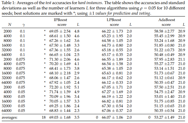
The following results reflect IPBoost's performance in hard instances. Note that by hard instances, we mean a binary classification problem with predefined labels. These examples are tailored to using the ±1 classification from learners. On every hard instance sample, IPBoost significantly outperforms both LPBoost and AdaBoost (although implementations depending on the libraries used have often caused results to differ slightly). For the considered instances the best value for the margin ρ was 0.05 for LPBoost and IPBoost; AdaBoost has no margin parameter. The accuracy reported is test accuracy recorded across various different walkthroughs of the algorithm, while [math]\displaystyle{ L }[/math] denotes the aggregate number of learners required to find the optimal learner, N is the number of points and [math]\displaystyle{ \gamma }[/math] refers to the noise level.

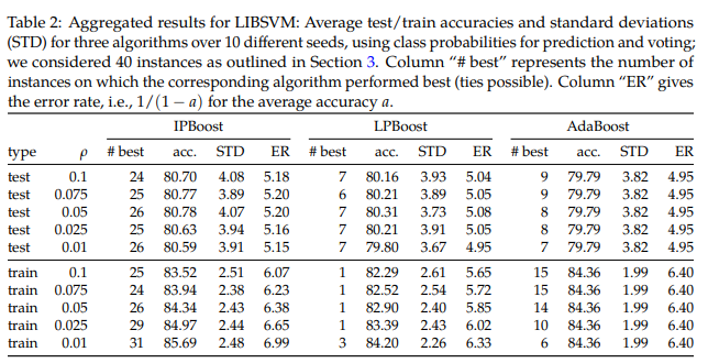
For the next table, the classification instances from LIBSVM data sets available at [1]. We report accuracies on the test set and train set, respectively. In each case, we report the averages of the accuracies over 10 runs with a different random seed and their standard deviations. We can see IPboost again outperforming LPBoost and AdaBoost significantly. Solving Integer Programming problems is no doubt more computationally expensive than traditional boosting methods like AdaBoost. The average run time of IPBoost (for ρ = 0.05) being 1367.78 seconds, as opposed to LPBoost's 164.35 seconds and AdaBoost's 3.59 seconds reflects exactly that. However, on the flip side, we gain much better stability in our results, as well as higher scores across the board for both training and test sets.

Conclusion
IP-boosting avoids the bad performance on well-known hard classes and improves upon LP-boosting and AdaBoost on the LIBSVM instances where even a few percent improvements are valuable. The major drawback is that the run time with the current implementation is much longer. Nevertheless, the algorithm can be improved in the future by approximating the intermediate LPs and deriving the tailored heuristics that generate decent primal solutions to save time.
The approach is suited very well to an offline setting in which training may take time and where even a small improvement is beneficial or when convex boosters have egregious behaviour. It can also be served as a tool to investigate the general performance of methods like this.
The IPBoost algorithm added extra complexity into basic boosting models to gain slight accuracy gain while greatly increased the time spent. It is 381 times slower compared to an AdaBoost model on a small dataset which makes the actual usage of this model doubtable. If we are supplied with a larger dataset with millions of records this model would take too long to complete. The base classifier choice was XGBoost which is too complicated for a base classifier, maybe try some weaker learners such as tree stumps to compare the result with other models. In addition, this model might not be accurate compared to the model-ensembling technique where each model utilizes a different algorithm.
I think IP Boost can be helpful in cases where a small improvement in accuracy is worth the additional computational effort involved. For example, there are applications in finance where predicting the movement of stock prices slightly more accurately can help traders make millions more. In such cases, investing in expensive computing systems to implement such boosting techniques can perhaps be justified.
Although the IPBoost can generate better results compared to the base boosting models such as AdaBoost. The time complexity of IPBoost is much higher than other models. Hence, it will be a problem to apply IPBoost to the real-world training data since those training data will be large and it's hard to deal with. Thus, we are left with the question that this IPBoost is only a little bit more accurate than the base boosting models but a lot more time complex. So is the model really worth it?
Critique
The introduction section should change the sentence"3. Push weight of the data ... will have a higher weight on those data that misclassified." to "... will have a higher weight on those misclassified data.
The column generation method is used when there are many variables compared to the number of constraints. If there are only a few variables compared to the number of limitations, using this method will not be very efficient.It would be better if the efficiency of different boosting models is tested.
In practice, AdaBoost & LP Boost are quite robust to overfitting. In a way, if you use simple weak learns stumps (1-level decision trees), then the algorithms are much less prone to overfitting. However, the noise level in the data, particularly for AdaBoost, is prone to overfitting noisy datasets. To avoid this use, regularized models (AdaBoostReg, LPBoost). Further, when in higher dimensional spaces, AdaBoost can suffer since it's just a linear combination of classifiers. You can use k-fold cross-validation to set the stopping parameter to improve this.
References
- Pfetsch, M. E., & Pokutta, S. (2020). IPBoost--Non-Convex Boosting via Integer Programming. arXiv preprint arXiv:2002.04679.
- Freund, Y., & Schapire, R. E. (1995, March). A desicion-theoretic generalization of on-line learning and an application to boosting. In European conference on computational learning theory (pp. 23-37). Springer, Berlin, Heidelberg. pdf