Being Bayesian about Categorical Probability

Presented By

Evan Li, Jason Pu, Karam Abuaisha, Nicholas Vadivelu

Introduction

Since the outputs of neural networks are not probabilities, Softmax (Bridle, 1990) is a staple for neural network’s performing classification--it exponentiates each logit then normalizes by the sum, giving a distribution over the target classes. However, networks with softmax outputs give no information about uncertainty (Blundell et al., 2015; Gal & Ghahramani, 2016), and the resulting distribution over classes is poorly calibrated (Guo et al., 2017), often giving overconfident predictions even when the classification is wrong. In addition, softmax also raises concerns about overfitting NNs due to its confident predictive behaviors(Xie et al., 2016; Pereyra et al., 2017). To achieve better generalization performance, this may require some effective regularization techniques.

Bayesian Neural Networks (BNNs; MacKay, 1992) can alleviate these issues, but the resulting posteriors over the parameters are often intractable. Approximations such as variational inference (Graves, 2011; Blundell et al., 2015) and Monte Carlo Dropout (Gal & Ghahramani, 2016) can still be expensive or give poor estimates for the posteriors. This work proposes a Bayesian treatment of the output logits of the neural network, treating the targets as a categorical random variable instead of a fixed label. This gives a computationally cheap way to get well-calibrated uncertainty estimates on neural network classifications.

Related Work

Using Bayesian Neural Networks is the dominant way of applying Bayesian techniques to neural networks. Many techniques have been developed to make posterior approximation more accurate and scalable, despite these, BNNs do not scale to the state of the art techniques or large data sets. There are techniques to explicitly avoid modeling the full weight posterior is more scalable, such as with Monte Carlo Dropout (Gal & Ghahramani, 2016) or tracking mean/covariance of the posterior during training (Mandt et al., 2017; Zhang et al., 2018; Maddox et al., 2019; Osawa et al., 2019). Non-Bayesian uncertainty estimation techniques such as deep ensembles (Lakshminarayanan et al., 2017) and temperature scaling (Guo et al., 2017; Neumann et al., 2018).

Preliminaries

Definitions

Let's formalize our classification problem and define some notations for the rest of this summary:

Dataset:

$$ \mathcal D = \{(x_i,y_i)\} \in (\mathcal X \times \mathcal Y)^N $$

General classification model

$$ f^W: \mathcal X \to \mathbb R^K $$

Softmax function:

$$ \phi(x): \mathbb R^K \to [0,1]^K \;\;|\;\; \phi_k(X) = \frac{\exp(f_k^W(x))}{\sum_{k \in K} \exp(f_k^W(x))} $$

Softmax activated NN:

$$ \phi \;\circ\; f^W: \chi \to \Delta^{K-1} $$

NN as a true classifier:

$$ arg\max_i \;\circ\; \phi_i \;\circ\; f^W \;:\; \mathcal X \to \mathcal Y $$

We'll also define the count function - a [math]\displaystyle{ K }[/math]-vector valued function that outputs the occurences of each class coincident with [math]\displaystyle{ x }[/math]: $$ c^{\mathcal D}(x) = \sum_{(x',y') \in \mathcal D} \mathbb y' I(x' = x) $$

Classification With a Neural Network

A typical loss function used in classification is cross-entropy. It's well known that optimizing [math]\displaystyle{ f^W }[/math] for [math]\displaystyle{ l_{CE} }[/math] is equivalent to optimizing for [math]\displaystyle{ l_{KL} }[/math]: $$ l_{KL}(W) = KL(\text{true distribution} \;||\; \text{distribution encoded by }NN(W)) $$ Let's introduce notation for the underlying (true) distributions of our problem. Let [math]\displaystyle{ (x_0,y_0) \sim (\mathcal X \times \mathcal Y) }[/math]: $$ \text{Full Distribution} = F(x,y) = P(x_0 = x,y_0 = y) $$ $$ \text{Marginal Distribution} = P(x) = F(x_0 = x) $$ $$ \text{Point Class Distribution} = P(y_0 = y \;|\; x_0 = x) = F_x(y) $$ Then we have the following factorization: $$ F(x,y) = P(x,y) = P(y|x)P(x) = F_x(y)F(x) $$ Substitute this into the definition of KL divergence: $$ = \sum_{(x,y) \in \mathcal X \times \mathcal Y} F(x,y) \log\left(\frac{F(x,y)}{\phi_y(f^W(x))}\right) $$ $$ = \sum_{x \in \mathcal X} F(x) \sum_{y \in \mathcal Y} F(y|x) \log\left( \frac{F(y|x)}{\phi_y(f^W(x))} \right) $$ $$ = \sum_{x \in \mathcal X} F(x) \sum_{y \in \mathcal Y} F_x(y) \log\left( \frac{F_x(y)}{\phi_y(f^W(x))} \right) $$ $$ = \sum_{x \in \mathcal X} F(x) KL(F_x \;||\; \phi\left( f^W(x) \right)) $$ As usual, we don't have an analytic form for [math]\displaystyle{ l }[/math] (if we did, this would imply we know [math]\displaystyle{ F_X }[/math] meaning we knew the distribution in the first place). Instead, estimate from [math]\displaystyle{ \mathcal D }[/math]: $$ F(x) \approx \hat F(x) = \frac{||c^{\mathcal D}(x)||_1}{N} $$ $$ F_x(y) \approx \hat F_x(y) = \frac{c^{\mathcal D}(x)}{|| c^{\mathcal D}(x) ||_1}$$ $$ \to l_{KL}(W) = \sum_{x \in \mathcal D} \frac{||c^{\mathcal D}(x)||_1}{N} KL \left( \frac{c^{\mathcal D}(x)}{||c^{\mathcal D}(x)||_1} \;||\; \phi(f^W(x)) \right) $$ The approximations [math]\displaystyle{ \hat F, \hat F_X }[/math] are often not very good though: consider a typical classification such as MNIST: we would never expect two handwritten digits to produce the exact same image. Hence [math]\displaystyle{ c^{\mathcal D}(x) }[/math] is (almost) always going to have a single index $1$ and the rest $0$. This has implications for our approximations: $$ \hat F(x) \text{ is uniform for all } x \in \mathcal D $$ $$ \hat F_x(y) \text{ is degenerate for all } x \in \mathcal D $$ This clearly has implications for overfitting: to minimize the KL term in [math]\displaystyle{ l_{KL}(W) }[/math] we want [math]\displaystyle{ \phi(f^W(x)) }[/math] to be very close to [math]\displaystyle{ \hat F_x(y) }[/math] at each point - this means that the loss function is in fact encouraging the neural network to output near degenerate distributions! One form of regularization to help this problem is called label smoothing. Instead of using the degenerate $F_x(y)$ as a target function, let's "smooth" it (by adding a scaled uniform distribution to it) so it's no longer degenerate: $$ F'_x(y) = (1-\lambda)\hat F_x(y) + \frac \lambda K \vec 1 $$

Method

The main technical proposal of the paper is a Bayesian framework to estimate the (former) target distribution [math]\displaystyle{ F_x(y) }[/math]. That is, we construct a posterior distribution of [math]\displaystyle{ F_x(y) }[/math] and use that as our new target distribution. We call it the belief matching (BM) framework.

Constructing Target Distribution

Recall that [math]\displaystyle{ F_x(y) }[/math] is a k-categorical probability distribution - it's PMF can be fully characterized by k numbers that sum to 1. Hence we can encode any such $F_x$ as a point in [math]\displaystyle{ \Delta^{k-1} }[/math]. We'll do exactly that - let's call this vecor [math]\displaystyle{ z }[/math]: $$ z \in \Delta^{k-1} $$ $$ \text{prior} = p_{z|x}(z) $$ $$ \text{conditional} = p_{y|z,x}(y) $$ $$ \text{posterior} = p_{z|x,y}(z) $$ Then if we perform inference: $$ p_{z|x,y}(z) \propto p_{z|x}(z)p_{y|z,x}(y) $$ The distribution chosen to model prior was [math]\displaystyle{ dir_K(\beta) }[/math]: $$ p_{z|x}(z) = \frac{\Gamma(||\beta||_1)}{\prod_{k=1}^K \Gamma(\beta_k)} \prod_{k=1}^K z_k^{\beta_k - 1} $$ Note that by definition of [math]\displaystyle{ z }[/math]: [math]\displaystyle{ p_{y|x,z} = z_y }[/math]. Since the Dirichlet is a conjugate prior to categorical distributions we have a convenient form for the mean of the posterior: $$ \bar{p_{z|x,y}}(z) = \frac{\beta + c^{\mathcal D}(x)}{||\beta + c^{\mathcal D}(x)||_1} \propto \beta + c^{\mathcal D}(x) $$ This is in fact a generalization of (uniform) label smoothing (label smoothing is a special case where [math]\displaystyle{ \beta = \frac 1 K \vec{1} }[/math]).

Representing Approximate Distribution

Our new target distribution is [math]\displaystyle{ p_{z|x,y}(z) }[/math] (as opposed to [math]\displaystyle{ F_x(y) }[/math]). That is, we want to construct an interpretation of our neural network weights to construct a distribution with support in [math]\displaystyle{ \Delta^{K-1} }[/math] - the NN can then be trained so this encoded distribution closely approximates [math]\displaystyle{ p_{z|x,y} }[/math]. Let's denote the PMF of this encoded distribution [math]\displaystyle{ q_{z|x}^W }[/math]. This is how the BM framework defines it: $$ \alpha^W(x) := \exp(f^W(x)) $$ $$ q_{z|x}^W(z) = \frac{\Gamma(||\alpha^W(x)||_1)}{\sum_{k=1}^K \Gamma(\alpha_k^W(x))} \prod_{k=1}^K z_{k}^{\alpha_k^W(x) - 1} $$ $$ \to Z^W_x \sim dir(\alpha^W(x)) $$ Apply [math]\displaystyle{ \log }[/math] then [math]\displaystyle{ \exp }[/math] to [math]\displaystyle{ q_{z|x}^W }[/math]: $$ q^W_{z|x}(z) \propto \exp \left( \sum_k (\alpha_k^W(x) \log(z_k)) - \sum_k \log(z_k) \right) $$ $$ \propto -l_{CE}(\phi(f^W(x)),z) + \frac{K}{||\alpha^W(x)||}KL(\mathcal U_k \;||\; z) $$ It can actually be shown that the mean of [math]\displaystyle{ Z_x^W }[/math] is identical to [math]\displaystyle{ \phi(f^W(x)) }[/math] - in other words, if we output the mean of the encoded distribution of our neural network under the BM framework, it is theoretically identical to a traditional neural network.

Distribution Matching

We now need a way to fit our approximate distribution from our neural network [math]\displaystyle{ q_{\mathbf{z | x}}^{\mathbf{W}} }[/math] to our target distribution [math]\displaystyle{ p_{\mathbf{z|x},y} }[/math]. The authors achieve this by maximizing the evidence lower bound (ELBO):

$$l_{EB}(\mathbf y, \alpha^{\mathbf W}(\mathbf x)) = \mathbb E_{q_{\mathbf{z | x}}^{\mathbf{W}}} \left[\log p(\mathbf {y | x, z})\right] - KL (q_{\mathbf{z | x}}^{\mathbf W} \; || \; p_{\mathbf{z|x}}) $$

Each term can be computed analytically:

$$\mathbb E_{q_{\mathbf{z | x}}^{\mathbf{W}}} \left[\log p(\mathbf {y | x, z})\right] = \mathbb E_{q_{\mathbf{z | x}}^{\mathbf W }} \left[\log z_y \right] = \psi(\alpha_y^{\mathbf W} ( \mathbf x )) - \psi(\alpha_0^{\mathbf W} ( \mathbf x )) $$

Where [math]\displaystyle{ \psi(\cdot) }[/math] represents the digamma function (logarithmic derivative of gamma function). Intuitively, we maximize the probability of the correct label. For the KL term:

$$KL (q_{\mathbf{z | x}}^{\mathbf W} \; || \; p_{\mathbf{z|x}}) = \log \frac{\Gamma(a_0^{\mathbf W}(\mathbf x)) \prod_k \Gamma(\beta_k)}{\prod_k \Gamma(\alpha_k^{\mathbf W}(x)) \Gamma (\beta_0)} + \sum_k (\alpha_k^{\mathbf W}(x)-\beta_k)(\psi(\alpha_k^{\mathbf W}(\mathbf x)) - \psi(\alpha_0^{\mathbf W}(\mathbf x)) $$

In the first term, for intuition, we can ignore [math]\displaystyle{ \alpha_0 }[/math] and [math]\displaystyle{ \beta_0 }[/math] since those just calibrate the distributions. Otherwise, we want the ratio of the products to be as close to 1 as possible to minimize the KL. In the second term, we want to minimize the difference between each individual [math]\displaystyle{ \alpha_k }[/math] and [math]\displaystyle{ \beta_k }[/math], scaled by the normalized output of the neural network.

This loss function can be used as a drop-in replacement for the standard softmax cross-entropy, as it has an analytic form and the same time complexity as typical softmax-cross entropy with respect to the number of classes ([math]\displaystyle{ O(K) }[/math]).

On Prior Distributions

We must choose our concentration parameter, $\beta$, for our dirichlet prior. We see our prior essentially disappears as [math]\displaystyle{ \beta_0 \to 0 }[/math] and becomes stronger as [math]\displaystyle{ \beta_0 \to \infty }[/math]. Thus, we want a small [math]\displaystyle{ \beta_0 }[/math] so the posterior isn't dominated by the prior. But, the authors claim that a small [math]\displaystyle{ \beta_0 }[/math] makes [math]\displaystyle{ \alpha_0^{\mathbf W}(\mathbf x) }[/math] small, which causes [math]\displaystyle{ \psi (\alpha_0^{\mathbf W}(\mathbf x)) }[/math] to be large, which is problematic for gradient based optimization. In practice, many neural network techniques aim to make [math]\displaystyle{ \mathbb E [f^{\mathbf W} (\mathbf x)] \approx \mathbf 0 }[/math] and thus [math]\displaystyle{ \mathbb E [\alpha^{\mathbf W} (\mathbf x)] \approx \mathbf 1 }[/math], which means making [math]\displaystyle{ \alpha_0^{\mathbf W}(\mathbf x) }[/math] small can be counterproductive.

So, the authors set [math]\displaystyle{ \beta = \mathbf 1 }[/math] and introduce a new hyperparameter [math]\displaystyle{ \lambda }[/math] which is multiplied with the KL term in the ELBO:

$$l^\lambda_{EB}(\mathbf y, \alpha^{\mathbf W}(\mathbf x)) = \mathbb E_{q_{\mathbf{z | x}}^{\mathbf{W}}} \left[\log p(\mathbf {y | x, z})\right] - \lambda KL (q_{\mathbf{z | x}}^{\mathbf W} \; || \; \mathcal P^D (\mathbf 1)) $$

This stabilizes the optimization, as we can tell from the gradients:

$$\frac{\partial l_{E B}\left(\mathbf{y}, \alpha^{\mathbf W}(\mathbf{x})\right)}{\partial \alpha_{k}^{\mathbf W}(\mathbf {x})}=\left(\tilde{\mathbf{y}}_{k}-\left(\alpha_{k}^{\mathbf W}(\mathbf{x})-\beta_{k}\right)\right) \psi^{\prime}\left(\alpha_{k}^{\mathbf{W}}(\boldsymbol{x})\right) -\left(1-\left(\alpha_{0}^{\boldsymbol{W}}(\boldsymbol{x})-\beta_{0}\right)\right) \psi^{\prime}\left(\alpha_{0}^{\boldsymbol{W}}(\boldsymbol{x})\right)$$

$$\frac{\partial l_{E B}^{\lambda}\left(\mathbf{y}, \alpha^{\mathbf{W}}(\mathbf{x})\right)}{\partial \alpha_{k}^{W}(\mathbf{x})}=\left(\tilde{\mathbf{y}}_{k}-\left(\tilde{\alpha}_{k}^{\mathbf W}(\mathbf{x})-\lambda\right)\right) \frac{\psi^{\prime}\left(\tilde{\alpha}_{k}^{\mathbf W}(\mathbf{x})\right)}{\psi^{\prime}\left(\tilde{\alpha}_{0}^{\mathbf W}(\mathbf{x})\right)} -\left(1-\left(\tilde{\alpha}_{0}^{W}(\mathbf{x})-\lambda K\right)\right)$$

As we can see, the first expression is affected by the magnitude of $\alpha^{\boldsymbol{W}}(\boldsymbol{x})$, whereas the second expression is not due to the [math]\displaystyle{ \frac{\psi^{\prime}\left(\tilde{\alpha}_{k}^{\mathbf W}(\mathbf{x})\right)}{\psi^{\prime}\left(\tilde{\alpha}_{0}^{\mathbf W}(\mathbf{x})\right)} }[/math] ratio.

Experiments

Throughout the experiments in this paper, the authors employ various models based on residual connections (He et al., 2016 [1]) which are the models used for benchmarking in practice. The only additions in the experiments are initial learning rate warm-up and gradient clipping which are extremely helpful for stable training of BM.

Generalization performance

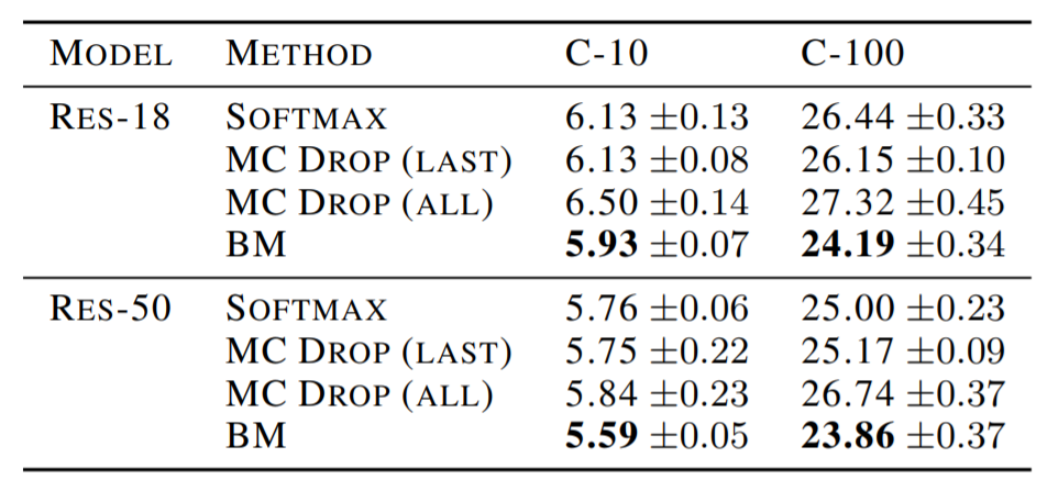
The paper compares the generalization performance of BM with softmax and MC dropout on CIFAR-10 and CIFAR-100 benchmarks.

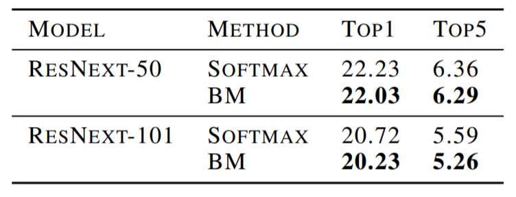
The next comparison was performed between BM and softmax on the ImageNet benchmark.

For both datasets and In all configurations, BM achieves the best generalization and outperforms softmax and MC dropout.

Regularization effect of prior

In theory, BM has 2 regularization effects: The prior distribution, which smooths the target posterior Averaging all of the possible categorical probabilities to compute the distribution matching loss The authors perform an ablation study to examine the 2 effects separately - removing the KL term in the ELBO removes the effect of the prior distribution. For ResNet-50 on CIFAR-100 and CIFAR-10 the resulting test error rates were 24.69% and 5.68% respectively.

This demonstrates that both regularization effects are significant since just having one of them improves the generalization performance compared to the softmax baseline, and having both improves the performance even more.

Impact of [math]\displaystyle{ \beta }[/math]

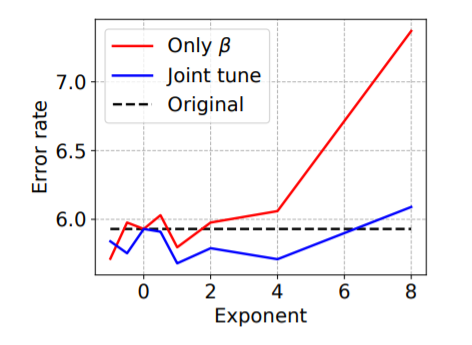
The effect of β on generalization performance is studied by training ResNet-18 on CIFAR-10 by tuning the value of β on its own, as well as jointly with λ. It was found that robust generalization performance is obtained for β ∈ [[math]\displaystyle{ e^{−1}, e^4 }[/math]] when tuning β on its own; and β ∈ [[math]\displaystyle{ e^{−4}, e^{8} }[/math]] when tuning β jointly with λ. The figure below shows a plot of the error rate with varying β.

Uncertainty Representation

One of the big advantages of BM is the ability to represent uncertainty about the prediction. The authors evaluate the uncertainty representation on in-distribution (ID) and out-of-distribution (OOD) samples.

ID uncertainty

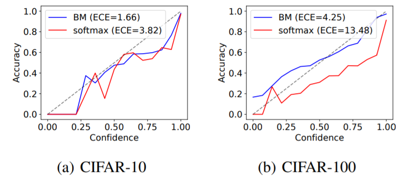
For ID (in-distribution) samples, calibration performance is measured, which is a measure of how well the model’s confidence matches its actual accuracy. This measure can be visualized using reliability plots and quantified using a metric called expected calibration error (ECE). ECE is calculated by grouping predictions into M groups based on their confidence score and then finding the absolute difference between the average accuracy and average confidence for each group. The figure below is a reliability plot of ResNet-50 on CIFAR-10 and CIFAR-100 with 15 groups. It shows that BM has a significantly better calibration performance than softmax since the confidence matches the accuracy more closely (this is also reflected in the lower ECE).

OOD uncertainty

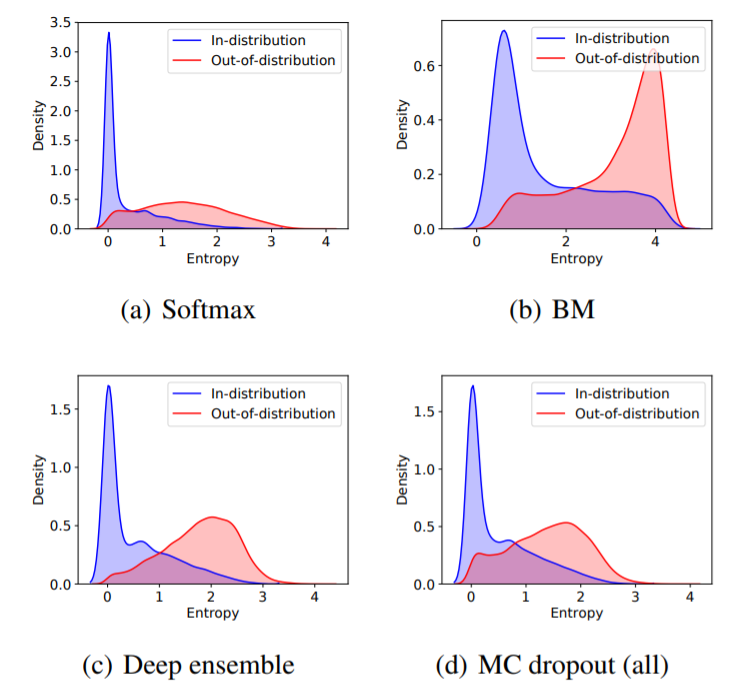
Here, the authors quantify uncertainty using predictive entropy - the larger the predictive entropy, the larger the uncertainty about a prediction.

The figure below is a density plot of the predictive entropy of ResNet-50 on CIFAR-10. It shows that BM provides significantly better uncertainty estimation compared to other methods since BM is the only method that has a clear peak of high predictive entropy for OOD samples which should have high uncertainty.

Transfer learning

Belief matching applies the Bayesian principle outside the neural network, which means it can easily be applied to already trained models. Thus, belief matching can be employed in transfer learning scenarios. The authors downloaded the ImageNet pre-trained ResNet-50 weights and fine-tuned the weights of the last linear layer for 100 epochs using an Adam optimizer.

This table shows the test error rates from transfer learning on CIFAR-10, Food-101, and Cars datasets. Belief matching consistently performs better than softmax.

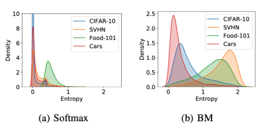
Belief matching was also tested for the predictive uncertainty for out of dataset samples based on CIFAR-10 as the in distribution sample. Looking at the figure below, it is observed that belief matching significantly improves the uncertainty representation of pre-trained models by only fine-tuning the last layer’s weights. Note that belief matching confidently predicts examples in Cars since CIFAR-10 contains the object category automobiles. In comparison, softmax produces confident predictions on all datasets. Thus, belief matching could also be used to enhance the uncertainty representation ability of pre-trained models without sacrificing their generalization performance.

Semi-Supervised Learning

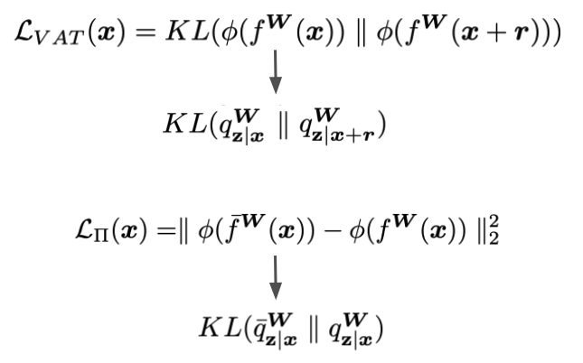
Belief matching’s ability to allow neural networks to represent rich information in their predictions can be exploited to aid consistency based loss function for semi-supervised learning. Consistency-based loss functions use unlabelled samples to determine where to promote the robustness of predictions based on stochastic perturbations. This can be done by perturbing the inputs (which is the VAT model) or the networks (which is the pi-model). Both methods minimize the divergence between two categorical probabilities under some perturbations, thus belief matching can be used by the following replacements in the loss functions. The hope is that belief matching can provide better prediction consistencies using its Dirichlet distributions.

The results of training on ResNet28-2 with consistency based loss functions on CIFAR-10 are shown in this table. Belief matching does have lower classification error rates compared to using a softmax.

Conclusion

Bayesian principles can be used to construct the target distribution by using the categorical probability as a random variable rather than a training label. This can be applied to neural network models by replacing only the softmax and cross-entropy loss, while improving the generalization performance and uncertainty estimation.

In the future, the authors would like to allow for more expressive distributions in the belief matching framework, such as logistic normal distributions to capture strong semantic similarities among class labels. Furthermore, using input dependent priors would allow for interesting properties that would aid imbalanced datasets and multi-domain learning.

Citations

[1] Bridle, J. S. Probabilistic interpretation of feedforward classification network outputs, with relationships to statistical pattern recognition. In Neurocomputing, pp. 227–236. Springer, 1990.

[2] Blundell, C., Cornebise, J., Kavukcuoglu, K., and Wierstra, D. Weight uncertainty in neural networks. In International Conference on Machine Learning, 2015.

[3] Gal, Y. and Ghahramani, Z. Dropout as a Bayesian approximation: Representing model uncertainty in deep learning. In International Conference on Machine Learning, 2016.

[4] Guo, C., Pleiss, G., Sun, Y., and Weinberger, K. Q. On calibration of modern neural networks. In International Conference on Machine Learning, 2017.

[5] MacKay, D. J. A practical Bayesian framework for backpropagation networks. Neural Computation, 4(3):448– 472, 1992.

[6] Graves, A. Practical variational inference for neural networks. In Advances in Neural Information Processing Systems, 2011.

[7] Mandt, S., Hoffman, M. D., and Blei, D. M. Stochastic gradient descent as approximate Bayesian inference. Journal of Machine Learning Research, 18(1):4873–4907, 2017.

[8] Zhang, G., Sun, S., Duvenaud, D., and Grosse, R. Noisy natural gradient as variational inference. In International Conference of Machine Learning, 2018.

[9] Maddox, W. J., Izmailov, P., Garipov, T., Vetrov, D. P., and Wilson, A. G. A simple baseline for Bayesian uncertainty in deep learning. In Advances in Neural Information Processing Systems, 2019.

[10] Osawa, K., Swaroop, S., Jain, A., Eschenhagen, R., Turner, R. E., Yokota, R., and Khan, M. E. Practical deep learning with Bayesian principles. In Advances in Neural Information Processing Systems, 2019.

[11] Lakshminarayanan, B., Pritzel, A., and Blundell, C. Simple and scalable predictive uncertainty estimation using deep ensembles. In Advances in Neural Information Processing Systems, 2017.

[12] Neumann, L., Zisserman, A., and Vedaldi, A. Relaxed softmax: Efficient confidence auto-calibration for safe pedestrian detection. In NIPS Workshop on Machine Learning for Intelligent Transportation Systems, 2018.