User:Bsharman

Risk prediction in life insurance industry using supervised learning algorithms

Presented By

Bharat Sharman, Dylan Li, Leonie Lu, Mingdao Li

Introduction

Risk assessment lies at the core of the life insurance industry. It is extremely important for companies to assess the risk of an application accurately to ensure that those submitted by actual low risk applicants are accepted, whereas applications submitted by high risk applicants are either rejected or placed aside for further review. The types of risks include but are not limited to, a person's smoking status, and family history (such as history of heart disease). If this is not the case, individuals with an extremely high risk profile might be issued policies, often leading to high insurance payouts and large losses for the company. Such a situation is called ‘Adverse Selection’, where individuals who are most likely to be issued a payout are in fact given a policy and those who are not as likely are not, thus causing the company to suffer losses as a result.

Traditionally, the process of underwriting (deciding whether or not to insure the life of an individual) has been done using actuarial calculations and judgements from underwriters. Actuaries group customers according to their estimated levels of risk determined from historical data. (Cummins J, 2013) However, these conventional techniques are time-consuming and it is not uncommon to take a month to issue a policy. They are expensive as a lot of manual processes need to be executed and a lot of data needs to be imported for the purpose of calculation.

Predictive analysis is an effective technique that simplifies the underwriting process to reduce policy issuance time and improve the accuracy of risk prediction. In life insurance, this approach is widely used in mortality rates modeling to help underwriters make decisions and improve the profitability of the business. In this paper, the authors used data from Prudential Life Insurance company and investigated the most appropriate data extraction method and the most appropriate algorithm to assess risk.

Literature Review

Before a life insurance company issues a policy, it must execute a series of underwriting related tasks (Mishr, 2016). These tasks involve gathering extensive information about the applicants. The insurer has to analyze the employment, medical, family, and insurance histories of the applicants and factor all of them into a complicated series of calculations to determine the risk rating of the applicants. On basis of this risk rating, premiums are calculated (Prince, 2016).

In a competitive marketplace, customers need policies to be issued quickly and long wait times can lead to them switch to other providers (Chen 2016). In addition, the costs of data gathering and analysis can be expensive. The insurance company bears the expenses of the medical examinations and if a policy lapses, then the insurer has to bear the losses of all these costs (J Carson, 2017). If the underwriting process uses predictive analytics, then the costs and time associated with many of these processes will be reduced significantly.

The key importance of a strong underwriting process for a life insurer is to avoid the risk of adverse selection. Adverse selection occurs in situations when an applicant has more knowledge about their health or conditions than the insurance company, and insurers can incur significant losses if they are systematically issuing policies to high-risk applicants due to this asymmetry of information. In order to avoid adverse selection, a strong classification system that correctly groups applicants into their appropriate risk levels is needed, and this is the motivation for this research.

Methods and Techniques

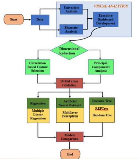
In Figure 1, the process flow of the analytics approach has been depicted. These stages will now be described in the following sections.

Description of the Dataset

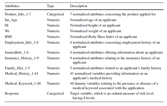
The data is obtained from the Kaggle competition hosted by the Prudential Life Insurance company. It has 59381 applications with 128 attributes. The attributes are continuous and discrete as well as categorical variables. The data attributes, their types and the description is shown in Table 1 below:

Data Pre-Processing

In the data preprocessing step, missing values in the data are either imputed or dropped and some of the attributes are either transformed to make the subsequent processing of data easier. This decision is made after determining the mechanism of missingness, that is if the data is Missing Completely at Random (MCAR), Missing at Random (MAR), or Missing Not at Random (MNAR).

Data Exploration using Visual Analytics

The Exploratory Data Analysis (EDA) is composed by uni-variate and bivariate analyses, which allows the researchers to understand different distributions' features. Visual analytics aims to gain insights of data structures by creating charts and graphs for the prediction models.

Dimensionality Reduction

In this paper, there are two methods that have been used for dimensionality reduction –

1.Correlation based Feature Selection (CFS): This is a feature selection method in which a subset of features from the original features is selected. In this method, the algorithm selects features from the dataset that are highly correlated with the output but are not correlated with each other. The user does not need to specify the number of features to be selected. The correlation values are calculated based on measures such as Pearson’s coefficient, minimum description length, symmetrical uncertainty, and relief.

2.Principal Components Analysis (PCA): PCA is a feature extraction method that transforms existing features into new sets of features such that the correlation between them is zero and these transformed features explain the maximum variability in the data.

PCA creates new features based on existing ones, while CFS only selects the best attributes based on the predictive power. Although PCA performs some feature engineering on attributes in data sets, the resulting new features are more complex to explain because it is difficult to derive meanings from principal components. On the other hand, CFS is easier to understand and interpret because the original features have not been merged or modified.

Supervised Learning Algorithms

The four algorithms that have been used in this paper are the following:

1.Multiple Linear Regression: In MLR, the relationship between the dependent and the two or more independent variables is predicted by fitting a linear model. The model parameters are calculated by minimizing the sum of squares of the errors, which captures the average distance between the predicted data points and observed data. The significance of the variables is determined by tests like the F test and the p-values.

2.REPTree: REPTree stands for reduced error pruning tree. It can build both classification and regression trees, depending on the type of the response variable. In this case, it uses regression tree logic and creates many trees across several iterations. This algorithm develops these trees based on the principles of information gain and variance reduction. At the time of pruning the tree, the algorithm uses the lowest mean square error to select the best tree.

3.Random Tree (Also known as the Random Forest): A random tree selects some of the attributes at each node in the decision tree and builds a tree based on random selection of data as well as attributes. Random Tree does not do pruning. Instead, it estimates class probabilities based on a hold-out set.

4.Artificial Neural Network: In a neural network, the inputs are transformed into outputs via a series of layered units where each of these units transforms the input received via a function into an output that gets further transmitted to units down the line. The weights that are used to weigh the inputs are improved after each iteration via a method called backpropagation in which errors propagate backward in the network and are used to update the weights to make the computed output closer to the actual output.

Experiments and Results

Missing Data Mechanism

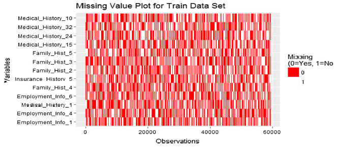
Attributes, where more than 30% of Data was missing, were dropped from the analysis. The data were tested for Missing Completely at Random (MCAR), one form of the nature of missing values using the Little Test. The null hypothesis that the missing data was completely random had a p-value of 0 meaning, MCAR was rejected. Then, all the variables were plotted to check how many missing values that they had, and the results are shown in the figure below:

The variables that have the most number of missing variables are plotted at the top and that have the least number of missing variables are plotted at the bottom of the y-axis in the figure above. Missing variables do not seem to have obvious patterns and therefore they are assumed to be Missing at Random (MAR), meaning the tendency for the variables to be missing is not related to the missing data but to the observed data.

Missing Data Imputation

Assuming that missing data follows a MAR pattern, multiple imputations are used as a technique to fill in the values of missing data. The steps involved in multiple imputation are the following:

Imputation: The imputation of the missing values is done over several steps and this results in a number of complete data sets. Imputation is usually done via a predictive model like linear regression to predict these missing values based on other variables in the data set.

Analysis: The complete data sets that are formed are analyzed and parameter estimates and standard errors are calculated.

Pooling: The analysis results are then integrated to form a final data set that is then used for further analysis.

Comparison of Feature Selection and Feature Extraction

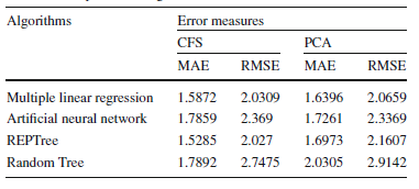
The Correlation-based Feature Selection (CFS) method was performed using the Waikato Environment for Knowledge Analysis. It was implemented using a Best-first search method on a CfsSubsetEval attribute evaluator. 33 variables were selected out of the total of 117 features. PCA was implemented via a Ranker Search Method using a Principal Components Attributes Evaluator. Out of the 117 features, those that had a standard deviation of more than 0.5 times the standard deviation of the first principal component were selected and this resulted in 20 features for further analysis. After dimensionality reduction, this reduced data set was exported and used for building prediction models using the four machine learning algorithms discussed before – REPTree, Multiple Linear Regression, Random Tree, and ANNs. The results are shown in the table below:

For CFS, the REPTree model had the lowest MAE and RMSE. For PCA, the Multiple Linear Regression Model had the lowest MAE as well as RMSE. So, for this dataset, it seems that overall, Multiple Linear Regression and REPTree Models are the two best ones with lowest error rates. In terms of dimensionality reduction, it seems that CFS is a better method than PCA for this data set as the MAE and RMSE values are lower for all ML methods except ANNs.

Conclusion and Further Work

Predictive Analytics in the Life Insurance Industry is enabling faster customer service and lower costs by helping automate the process of Underwriting, thereby increasing satisfaction and loyalty. In this study, the authors analyzed data obtained from Prudential Life Insurance to predict risk scores via Supervised Machine Learning Algorithms. The data was first pre-processed to first replace the missing values. Attributes having more than 30% of missing data were eliminated from the analysis. Two methods of dimensionality reduction – CFS and PCA were used and the number of attributes used for further analysis was reduced to 33 and 20 via these two methods. The Machine Learning Algorithms that were implemented were – REPTree, Random Tree, Multiple Linear Regression, and Artificial Neural Networks. Model validation was performed via ten-fold cross-validation. The performance of the models was evaluated using MAE and RMSE measures. Using the PCA method, Multiple Linear Regression showed the best results with MAE and RMSE values of 1.64 and 2.06 respectively. With CFS, REPTree had the highest accuracy with MAE and RMSE values of 1.52 and 2.02 respectively. Further work can be directed towards dealing with all the variables rather than deleting the ones where more than 30% of the values are missing. Customer segmentation, i.e. grouping customers based on their profiles can help companies come up with a customized policy for each group. This can be done via unsupervised algorithms like clustering. Work can also be done to make the models more explainable especially if we are using PCA and ANNs to analyze data. We can also get indirect data about the prospective applicant like their driving behavior, education record, etc to see if these attributes contribute to better risk profiling than the already available data.

Critiques

The project built multiple models and had utilized various methods to evaluate the result. They could potentially ensemble the prediction, such as averaging the result of the different models, to achieve a better accuracy result. Another method is model stacking, we can input the result of one model as input into another model for better results. However, they do have some major setbacks: sometimes, the result could be effect negatively (ie: increase the RMSE). In addition, if the improvement is not prominent, it would make the process much more complex thus cost time and effort. In a research setting, stacking and ensembling are definitely worth a try. In a real-life business case, it is more of a trade-off between accuracy and effort/cost.

In this application, it is not essentially the same thing as classify risky as non-risky or vice versa, if the model misclassified a risky data as non-risky, it may create a large loss to the insurance companies. It is recommended that this issue could be carefully taken care of during the model selection.

This project only used unsupervised dimensionality reduction techniques to analyze the data and did not explore supervised methods such as linear discriminant analysis, quadratic discriminant analysis, Fisher discriminant analysis, or supervised PCA. The supervisory signal could've been the normalized risk score, which determines whether someone is granted the policy. The supervision might have provided insight on factors contributing to risk that would not have been captured with unsupervised methods.

In addition, the dimensionality reduction techniques seem to contradict each other. If we do select features based on their correlation, there is no need to do further PCA on the dataset. Even if we perform PCA, the resulting columns would have a similar number of columns compared to the original ones and it would lose interpretability of the features, which is crucial in real-life practices.

Some of the models mentioned in this article require a large amount of data to perform well (e.g. neural network and tree-based algorithm). In a practical sense, a direct insurer may not have enough data (for certain lines of businesses) to train these models, overfitting could be a serious problem. The computational cost could be another critical issue. On a small dataset, Bayesian methods can be used to incorporate prior information into statistical models to obtain more refined inference.

Attributes that have more than 30% missing data were dropped. The disadvantage of this is that the dropped variable might affect other variables in the dataset. An alternative approach to dealing with missing data would be the use of Neural Networks, eliminating the need for deletion or imputation depending on the mechanism missingness (Smieja et al 2018).

The project contains multiple models and requires a lot of data to execute the algorithm well, but the data set is entirely from an insurance company. These data will have incompleteness and one-sided factors leading to inaccurate results. In the summary part, no specific conclusions and future work are mentioned, and the structure is not obvious and requires specific explanation.

The project provides an idea for the insurance industry to analyze risks. For the model selection part, I am thinking that it might be an idea to involve more complicated models to detect the baseline for the datasets. Besides, applying more complicated models might work as a justification for the feature selection correctness.

For sections titled "Missing Data Imputation" and "Missing Data Mechanism", it would be highly significant for the authors to provide more details regarding the experimental results. For instance, the authors mentioned that the null hypothesis which the missing data was completely random had a p-value of 0 meaning, MCAR was rejected. However, no relevant calculation or explanation has been provided to justify such conclusion.

In the Data pre-processing part, the author did not specify what are MCAR, MAR, and MNAR. Technically speaking, MCAR stands for the missing values are like a random sample of all the cases in the feature. MAR stands for missing values can be predicted using the observed data. And MNAR means the missing values cannot be explained by the observed part of the data.

This project used supervised Machine learning to predict risked score. In the prepossessing data step, the author used MCAR, MAR, MNAR methods and drop roughly 30% missing data, which might leads the insufficient training data for the model. Meanwhile, all the data came from the insurance company which is subjective. Moreover, it would be better if the data pre-processing part to indicate what will be the main difference among MCAR, MAR and MNAR methods.

As mentioned in the previous critique, having risky and non-risky as the output is not neccessarily true, not just for the company, but also for the consumer as us.

References

Chen, T. (2016). Corporate reputation and financial performance of Life Insurers. Geneva Papers Risk Insur Issues Pract, 378-397.

Cummins J, S. B. (2013). Risk classification in Life Insurance. Springer 1st Edition.

J Carson, C. E. (2017). Sunk costs and screening: two-part tariffs in life insurance. SSRN Electron J, 1-26.

Jayabalan, N. B. (2018). Risk prediction in life insurance industry using supervised learning algorithms. Complex & Intelligent Systems, 145-154.

Mishr, K. (2016). Fundamentals of life insurance theories and applications. PHI Learning Pvt Ltd.

Prince, A. (2016). Tantamount to fraud? Exploring non-disclosure of genetic information in life insurance applications as grounds for policy recession. Health Matrix, 255-307.

Śmieja, M., Struski, Ł., Tabor, J., Zieliński, B., & Spurek, P. (2018). Processing of missing data by neural networks. In Advances in Neural Information Processing Systems (pp. 2719-2729).