Adacompress: Adaptive compression for online computer vision services
Presented by
Ahmed Hussein Salamah
Introduction
Big data and deep learning have been merged to create the great success of artificial intelligence which increases the burden on the network's speed, computational complexity, and storage in many applications. The image Classification task is one of the most important computer vision tasks which has shown a high dependency on Deep Neural Networks to improve their performance in many applications. Recently, they tend to use different image classification models on the cloud just to share the computational power between the different users as mentioned in this paper (e.g., SenseTime, Baidu Vision and Google Vision, etc.). Most of the researchers in the literature work to improve the structure and increase the depth of DNNs to achieve better performance from the point of how the features are represented and crafted using Conventional Neural Networks (CNNs). As the most well-known image classification datasets (e.g. ImageNet) are compressed using JPEG and this compression technique is optimized for Human Visual System (HVS) but not the machines (i.e. DNNs), so to be aligned with HVS the authors have to reconfigure the JPEG while maintaining the same classification accuracy.
Why is image compression important?
Image compression is crucial in deep learning because we want the image data to take up less disk space and can be loaded faster. Compared to the lossless compression PNG, which preserves the original image data, JPEG is a lossy form of compression meaning some information will be lost though for the benefit of an improved compression ratio. Therefore, it is important to develop deep learning model-based image compression methods which reduce data size without jeopardizing classification accuracy. Some examples of this type of image compression includes the LSTM-based approach proposed by Google [9], the transformation-based method from New York University [10], the autoencoder-based approach by Twitter [11], etc.
Methodology
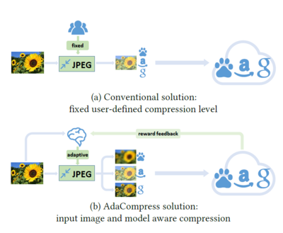
One of the major parameters that can be changed in the JPEG pipeline is the quantization table, which is the main source of artifacts added in the image to make it lossless compression as shown in [1, 4]. The authors got motivated to change the JPEG configuration to optimize the uploading rate of different cloud computer vision without considering pre-knowledge of the original model and dataset. In contrast to the authors in [2, 3, 5] where they adjust the JPEG configuration by retraining the parameters or according to the structure of the model. They considered the lack of undefined quantization level which decreases the image rate and quality but the deep learning model can still recognize it as shown in [4]. The authors in [1] used Deep Reinforcement learning (DRL) in an online manner to choose the quantization level to upload an image to the cloud for the computer vision model and this is the only approach to design an adaptive JPEG based on RL mechanism.
The approach is designed based on an interactive training environment which represents any computer vision cloud services, then they needed a tool to evaluate and predict the performance of quantization level on an uploaded image, so they used a deep Q neural network agent. They feed the agent with a reward function which considers two optimization parameters, accuracy and image size. It works as iterative behavior interacting with the environment. The environment is exposed to different images with different virtual redundant information that needs an adaptive solution for each image to select the suitable compression level for the model. Thus, they designed an explore-exploit mechanism to train the agent on different scenery which is designed in deep Q agent as an inference-estimate-retain mechanism to restart the training procedure for each image. The authors verify their approach by providing some analysis and insight using Grad-Cam [8] by showing some patterns of how a compression level is chosen for each image with its own corresponding quality factor. Each image shows a different response when shown to a deep learning model. In general, images are more sensitive to compression if they have large smooth areas, while those with complex textures are more robust to compression.
What is a quantization table?
Before getting to the quantization table first look at the basic architecture of JPEG's baseline system. This has 4 blocks, which are FDCT (Fast Discrete Cosine Transformation), quantizer, statistical model, and entropy encoder. The FCDT block takes an input image separated into [math]\displaystyle{ n \times n }[/math] blocks and applies a discrete cosine transformation creating DCT terms. These DCT terms are values from a relatively large discrete set that will be then mapped through the process of quantization to a smaller discrete set. This is accomplished with a quantization table at the quantizer block, which is designed to preserve low-frequency information at the cost of the high-frequency information. This preference for low frequency information is made because losing high frequency information isn't as impactful to the image when perceived by a humans visual system.
Problem Formulation
The authors formulate the problem by referring to the cloud deep learning service as [math]\displaystyle{ \vec{y}_i = M(x_i) }[/math] to predict results list [math]\displaystyle{ \vec{y}_i }[/math] for an input image [math]\displaystyle{ x_i }[/math], and for reference input [math]\displaystyle{ x \in X_{\rm ref} }[/math] the output is [math]\displaystyle{ \vec{y}_{\rm ref} = M(x_{\rm ref}) }[/math]. It is referred [math]\displaystyle{ \vec{y}_{\rm ref} }[/math] as the ground truth label and also [math]\displaystyle{ \vec{y}_c = M(x_c) }[/math] for compressed image [math]\displaystyle{ x_{c} }[/math] with quality factor [math]\displaystyle{ c }[/math].
\begin{align} \tag{1} \label{eq:accuracy}
\mathcal{A} =& \sum_{k}\min_jd(l_j, g_k) \\
& l_j \in \vec{y}_c, \quad j=1,...,5 \nonumber \\
& g_k \in \vec{y}_{\rm ref}, \quad k=1, ..., {\rm length}(\vec{y}_{\rm ref}) \nonumber \\
& d(x, y) = 1 \ \text{if} \ x=y \ \text{else} \ 0 \nonumber
\end{align}
The authors divided the used datasets according to their contextual group [math]\displaystyle{ X }[/math] according to [6] and they compare their results using compression ratio [math]\displaystyle{ \Delta s = \frac{s_c}{s_{\rm ref}} }[/math], where [math]\displaystyle{ s_{c} }[/math] is the compressed size and [math]\displaystyle{ s_{\rm ref} }[/math] is the original size, and accuracy metric [math]\displaystyle{ \mathcal{A}_c }[/math] which is calculated based on the hamming distance of Top-5 of the output of softmax probabilities for both original and compressed images as shown in Eq. \eqref{eq:accuracy}. In the RL designing stage, continuous numerical vectors are represented as the input features to the DRL agent which is Deep Q Network (DQN). The challenges of using this approach are: (1) The state space of RL is too large to cover, so the neural network is typically constructed with more layers and nodes, which makes the DRL agent hard to converge and the training time-consuming; (2) The DRL always starts with a random initial state, but it needs to find a higher reward before starting the training of the DQN. However, the sparse reward feedback resulted from a random initialization makes learning difficult. The authors solve this problem by using a pre-trained small model called MobileNetV2 as a feature extractor [math]\displaystyle{ \mathcal{E} }[/math] for its ability in lightweight and image classification, and it is fixed during training the Q Network [math]\displaystyle{ \phi }[/math]. The last convolution layer of [math]\displaystyle{ \mathcal{E} }[/math] is connected as an input to the Q Network [math]\displaystyle{ \phi }[/math], so by optimizing the parameters of Q network [math]\displaystyle{ \phi }[/math], the RL agent's policy is updated.
Reinforcement learning framework
This paper [1] described the reinforcement learning problem as [math]\displaystyle{ \{\mathcal{X}, M\} }[/math] to be emulator environment, where [math]\displaystyle{ \mathcal{X} }[/math] is defining the contextual information created as an input from the user [math]\displaystyle{ x }[/math] and [math]\displaystyle{ M }[/math] is the backend cloud model. Each RL frame must be defined by action and state, the action is known by 10 discrete quality levels ranging from 5 to 95 by step size of 10 and the state is feature extractor's output [math]\displaystyle{ \mathcal{E}(J(\mathcal{X}, c)) }[/math], where [math]\displaystyle{ J(\cdot) }[/math] is the JPEG output at specific quantization level [math]\displaystyle{ c }[/math]. They found the optimal quantization level at time [math]\displaystyle{ t }[/math] is [math]\displaystyle{ c_t = {\rm argmax}_cQ(\phi(\mathcal{E}(f_t)), c; \theta) }[/math], where [math]\displaystyle{ Q(\phi(\mathcal{E}(f_t)), c; \theta) }[/math] is action-value function, [math]\displaystyle{ \theta }[/math] indicates the parameters of Q network [math]\displaystyle{ \phi }[/math]. In the training stage of RL, the goal is to minimize a loss function [math]\displaystyle{ L_i(\theta_i) = \mathbb{E}_{s, c \sim \rho (\cdot)}\Big[\big(y_i - Q(s, c; \theta_i)\big)^2 \Big] }[/math] that changes at each iteration [math]\displaystyle{ i }[/math] where [math]\displaystyle{ s = \mathcal{E}(f_t) }[/math] and [math]\displaystyle{ f_t }[/math] is the output of the JPEG, and [math]\displaystyle{ y_i = \mathbb{E}_{s' \sim \{\mathcal{X}, M\}} \big[ r + \gamma \max_{c'} Q(s', c'; \theta_{i-1}) \mid s, c \big] }[/math] is the target that has a probability distribution [math]\displaystyle{ \rho(s, c) }[/math] over sequences [math]\displaystyle{ s }[/math] and quality level [math]\displaystyle{ c }[/math] at iteration [math]\displaystyle{ i }[/math], and [math]\displaystyle{ r }[/math] is the feedback reward.
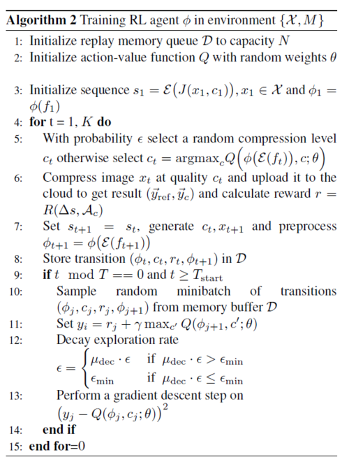
The framework get more accurate estimation from a selected action when the distance of the target and the action-value function's output [math]\displaystyle{ Q(\cdot) }[/math] is minimized. As a results, no feedback signal can tell that an episode has finished a condition value [math]\displaystyle{ T }[/math] that satisfies [math]\displaystyle{ t \geq T_{\rm start} }[/math] to guarantee to store enough transitions in the memory buffer [math]\displaystyle{ D }[/math] to train on. To create this transitions for the RL agent, random trials are collected to observe environment reaction. After fetching some trials from the environment with their corresponding rewards, this randomness is decreased as the agent is trained to minimize the loss function [math]\displaystyle{ L }[/math] as shown in the Algorithm below. Thus, it optimizes its actions on a minibatch from [math]\displaystyle{ \mathcal{D} }[/math] to be based on historical optimal experience to train the compression level predictor [math]\displaystyle{ \phi }[/math]. When this trained predictor [math]\displaystyle{ \phi }[/math] is deployed, the RL agent will drive the compression engine with the adaptive quality factor [math]\displaystyle{ c }[/math] corresponding to the input image [math]\displaystyle{ x_{i} }[/math].
The interaction between the agent and environment [math]\displaystyle{ \{\mathcal{X}, M\} }[/math] is evaluated using the reward function, which is formulated, by selecting an appropriate action of quality factor [math]\displaystyle{ c }[/math], to be directly proportional to the accuracy metric [math]\displaystyle{ \mathcal{A}_c }[/math], and inversely proportional to the compression rate [math]\displaystyle{ \Delta s = \frac{s_c}{s_{\rm ref}} }[/math]. As a result, the reward function is given by [math]\displaystyle{ R(\Delta s, \mathcal{A}) = \alpha \mathcal{A} - \Delta s + \beta }[/math], where [math]\displaystyle{ \alpha }[/math] and [math]\displaystyle{ \beta }[/math] to form a linear combination.
Inference-Estimate-Retrain Mechanism
The system diagram, AdaCompress, is shown in figure 3 in contrast to the existing modules. When the AdaCompress is deployed, the input images scenery context [math]\displaystyle{ \mathcal{X} }[/math] may change, in this case the RL agent’s compression selection strategy may cause the overall accuracy to decrease. So, in order to solve this issue, the estimator will be invoked with probability [math]\displaystyle{ p_{est} }[/math]. This will be done by generating a random value [math]\displaystyle{ \eps \in (0,1) \lt \math\gt and the estimator will be invoked if \lt math\gt \eps \lt p_{est} }[/math]. Then AdaCompress will upload both the original image and the compressed image to fetch their labels. The accuracy will then be calculated and the transition, which also includes the accuracy in this step, will be stored in the memory buffer. Comparing recent the n steps' average accuracy with earliest average accuracy, the estimator will then invoke the RL training kernel to retrain if the recent average accuracy is much lower than the initial average accuracy.
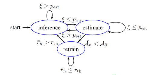
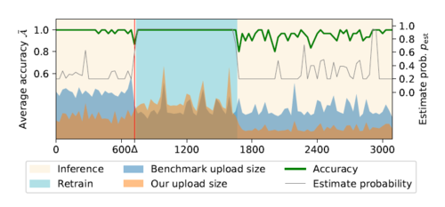
The authors solved the change in the scenery at the inference phase that might cause learning to diverge by introducing running-estimate-retain mechanism. They introduced estimator with probability [math]\displaystyle{ p_{\rm est} }[/math] that changes in an adaptive way and it is compared a generated random value [math]\displaystyle{ \xi \in (0,1) }[/math]. As shown in Figure 2, Adacompression is switching between three states in an adaptive way as will be shown in the following sections.
Inference State
The inference state is running most of the time at which the deployed RL agent is trained and used to predict the compression level [math]\displaystyle{ c }[/math] to be uploaded to the cloud with minimum uploading traffic load. The agent will eventually switch to the estimator stage with probability [math]\displaystyle{ p_{\rm est} }[/math] so it will be robust to any change in the scenery to have a stable accuracy. The [math]\displaystyle{ p_{\rm est} }[/math] is fixed at the inference stage but changes in an adaptive way as a function of accuracy gradient in the next stage. In estimator state, there will be a trade off between the objective of reducing upload traffic and the risk of changing the scenery, an accuracy-aware dynamic [math]\displaystyle{ p'_{\rm est} }[/math] is designed to calculate the average accuracy [math]\displaystyle{ \mathcal{A}_n }[/math] after running for defined [math]\displaystyle{ N }[/math] steps according to Eq. \ref{eqn:accuracy_n}. \begin{align} \tag{2} \label{eqn:accuracy_n} \bar{\mathcal{A}_n} &= \begin{cases} \frac{1}{n}\sum_{i=N-n}^{N} \mathcal{A}_i & \text{ if } N \geq n \\ \frac{1}{n}\sum_{i=1}^{n} \mathcal{A}_i & \text{ if } N < n \end{cases} \end{align}
Estimator State
The estimator state is executed when [math]\displaystyle{ \xi \leq p_{\rm est} }[/math] is satisfied , where the uploaded traffic is increased as the both the reference image [math]\displaystyle{ x_{ref} }[/math] and compressed image [math]\displaystyle{ x_{i} }[/math] are uploaded to the cloud to calculate [math]\displaystyle{ \mathcal{A}_i }[/math] based on [math]\displaystyle{ \vec{y}_{\rm ref} }[/math] and [math]\displaystyle{ \vec{y}_i }[/math]. It will be stored in the memory buffer [math]\displaystyle{ \mathcal{D} }[/math] as a transition [math]\displaystyle{ (\phi_i, c_i, r_i, \mathcal{A}_i) }[/math] of trial [math]\displaystyle{ i }[/math]. The estimator will not be anymore suitable for the latest [math]\displaystyle{ n }[/math] step when the average accuracy [math]\displaystyle{ \bar{\mathcal{A}}_n }[/math] is lower than the earliest [math]\displaystyle{ n }[/math] steps of the average [math]\displaystyle{ \mathcal{A}_0 }[/math] in the memory buffer [math]\displaystyle{ \mathcal{D} }[/math]. Consequently, [math]\displaystyle{ p_{\rm est} }[/math] should be changed to higher value to make the estimate stage frequently happened.It is obviously should be a function in the gradient of the average accuracy [math]\displaystyle{ \bar{\mathcal{A}}_n }[/math] in such a way to fell the buffer memory [math]\displaystyle{ \mathcal{D} }[/math] with some transitions to retrain the agent at a lower average accuracy [math]\displaystyle{ \bar{\mathcal{A}}_n }[/math]. The authors formulate [math]\displaystyle{ p'_{\rm est} = p_{\rm est} + \omega \nabla \bar{\mathcal{A}} }[/math] and [math]\displaystyle{ \omega }[/math] is a scaling factor. Initially the estimated probability [math]\displaystyle{ p_0 }[/math] will be a function of [math]\displaystyle{ p_{\rm est} }[/math] in the general form of [math]\displaystyle{ p_{\rm est} = p_0 + \omega \sum_{i=0}^{N} \nabla \bar{\mathcal{A}_i} }[/math].
Retrain State
In retrain state, the RL agent is trained to adapt on the change of the input scenery on the stored transitions in the buffer memory [math]\displaystyle{ \mathcal{D} }[/math]. The retain stage is finished at the recent [math]\displaystyle{ n }[/math] steps when the average reward [math]\displaystyle{ \bar{r}_n }[/math] is higher than a defined [math]\displaystyle{ r_{th} }[/math] by the user. Afterward, a new retraining stage should be prepared by saving new next transitions after flushing the old buffer memory [math]\displaystyle{ \mathcal{D} }[/math]. The authors supported their compression choice for different cloud application environments by providing some insights by introducing a visualization algorithm [8] to some images with their corresponding quality factor [math]\displaystyle{ c }[/math]. The visualization shows that the agent chooses a certain quantization level [math]\displaystyle{ c }[/math] based on the visual textures in the image at the different regions. For an instant, a low-quality factor is selected for the rough central region so there is a smooth area surrounded it but for the surrounding smooth region, the agent chooses a relatively higher quality rather than the central region.
Results
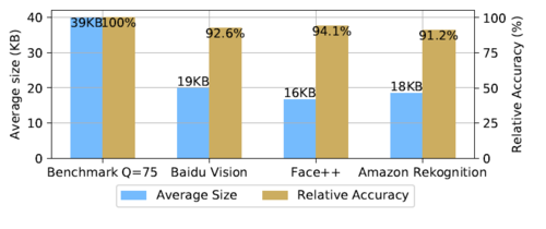
The authors reported in Figure 3, 3 different cloud services compared to the benchmark images. It is shown that more than the half of the upload size while roughly preserving the top-5 accuracy calculated by using A with an average of 7% proving the efficiency of the design. In Figure 4, it shows the inference-estimate-retain mechanism as the x-axis indicates steps, while [math]\displaystyle{ \Delta }[/math] mark on [math]\displaystyle{ x }[/math]-axis is reveal as a change in the scenery. In Figure 4, the estimating probability [math]\displaystyle{ p_{\rm est} }[/math] and the accuracy are inversely proportion as the accuracy drops below the initial value the [math]\displaystyle{ p_{\rm est} }[/math] increase adaptive as it considers the accuracy metric [math]\displaystyle{ \mathcal{A}_c }[/math] each action [math]\displaystyle{ c }[/math] making the average accuracy to decrease in the next estimations. At the red vertical line, the scenery started to change and [math]\displaystyle{ Q }[/math] Network start to retrain to adapt the the agent on the current scenery. At retrain stage, the output result is always use from the reference image's prediction label [math]\displaystyle{ \vec{y}_{\rm ref} }[/math]. Also, they plotted the scaled uploading data size of the proposed algorithm and the overhead data size for the benchmark is shown in the inference stage. After the average accuracy became stable and high, the transmission is reduced by decreasing the [math]\displaystyle{ p_{\rm est} }[/math] value. As a result, [math]\displaystyle{ p_{\rm est} }[/math] and [math]\displaystyle{ \mathcal{A} }[/math] will be always equal to 1. During this stage, the uploaded file is more than the conventional benchmark. In the inference stage, the uploaded size is halved as shown in both Figures 3, 4.
Conclusion
Most of the research focused on modifying the deep learning model instead of dealing with the currently available approaches. The authors succeed in defining the compression level for each uploaded image to decrease the size and maintain the top-5 accuracy in a robust manner even the scenery is changed. In my opinion, Eq. \eqref{eq:accuracy} is not defined well as I found it does not really affect the reward function. Also, they did not use the whole validation set from ImageNet which raises the question of what is the higher file size that they considered from in the mention current set. In addition, if they considered the whole data set, should we expect the same performance for the mechanism.
Critiques
The authors used a pre-trained model as a feature extractor to select a Quality Factor (QF) for the JPEG. I think what would be missing that they did not report the distribution of each of their span of QFs as it is important to understand which one is expected to contribute more. In my video, I have done one experiment using Inception-V3 to understand if it is possible to get better accuracy. I found that it is possible by using the inception model as a pre-trained model to choose a lower QF, but as well known that the mobile models are shallower than the inception models which make it less complex to run on edge devices. I think it is possible to achieve at least the same accuracy or even more if we replaced the mobile model with the inception. Another point, the authors did not run their approach on a complete database like ImageNet, they only included a part of two different datasets. I know they might have limitations in the available datasets to test like CIFARs, as they are not totally comparable from the resolution perspective for the real online computer vision services work with higher resolutions.
Source Code
https://github.com/AhmedHussKhalifa/AdaCompress
References
[1] Hongshan Li, Yu Guo, Zhi Wang, Shutao Xia, and Wenwu Zhu, “Adacompress: Adaptive compression for online computer vision services,” in Proceedings of the 27th ACM International Conference on Multimedia, New York, NY, USA, 2019, MM ’19, pp. 2440–2448, ACM.
[2] Zihao Liu, Tao Liu, Wujie Wen, Lei Jiang, Jie Xu, Yanzhi Wang, and Gang Quan, “DeepN-JPEG: A deep neural network favorable JPEG-based image compression framework,” in Proceedings of the 55th Annual Design Automation Conference. ACM, 2018, p. 18.
[3] Lionel Gueguen, Alex Sergeev, Ben Kadlec, Rosanne Liu, and Jason Yosinski, “Faster neural networks straight from jpeg,” in Advances in Neural Information Processing Systems, 2018, pp. 3933–3944.
[4] Kresimir Delac, Mislav Grgic, and Sonja Grgic, “Effects of jpeg and jpeg2000 compression on face recognition,” in Pattern Recognition and Image Analysis, Sameer Singh, Maneesha Singh, Chid Apte, and Petra Perner, Eds., Berlin, Heidelberg, 2005, pp. 136–145, Springer Berlin Heidelberg.
[5] Robert Torfason, Fabian Mentzer, Eirikur Agustsson, Michael Tschannen, Radu Timofte, and Luc Van Gool, “Towards image understanding from deep compression without decoding,” 2018.
[6] Seungyeop Han, Haichen Shen, Matthai Philipose, Sharad Agarwal, Alec Wolman, and Arvind Krishnamurthy, “Mcdnn: An approximation-based execution framework for deep stream processing under resource constraints,” in Proceedings of the 14th Annual International Conference on Mobile Systems, Applications, and Services, New York, NY, USA, 2016, MobiSys ’16, pp. 123–136, ACM.
[7] Mark Sandler, Andrew G. Howard, Menglong Zhu, Andrey Zhmoginov, and Liang-Chieh Chen, “Inverted residuals and linear bottlenecks: Mobile networks for classification, detection and segmentation,” CoRR, vol. abs/1801.04381, 2018.
[8] Ramprasaath R. Selvaraju, Abhishek Das, Ramakrishna Vedantam, Michael Cogswell, Devi Parikh, and Dhruv Batra, “Grad-cam: Why did you say that? visual explanations from deep networks via gradient-based localization,” CoRR, vol. abs/1610.02391, 2016.
[9] George Toderici, Sean M. O'Malley, Sung Jin Hwang, Damien Vincent, David Minnen, Shumeet Baluja, Michele Covell, Rahul Sukthankarm, Variable Rate Image Compression with Recurrent Neural Networks, ICLR 2016, arXiv:1511.06085
[10] Johannes Ballé, Valero Laparra, Eero P. Simoncelli, End-to-end Optimized Image Compression, ICLR 2017, arXiv:1611.01704
[11] Lucas Theis, Wenzhe Shi, Andrew Cunningham, Ferenc Huszár, Lossy Image Compression with Compressive Autoencoders, ICLR 2017, arXiv:1703.00395