User:J46hou
DROCC: Deep Robust One-Class Classification
Presented by
Jinjiang Lian, Yisheng Zhu, Jiawen Hou, Mingzhe Huang
Introduction
In this work, we study “one-class” classification, where the goal is to obtain accurate discriminators for a special class. Popular uses of this technique include anomaly detection where we are interested in detecting outliers. Anomaly detection is a well-studied area of research, however, the conventional approach of modeling with typical data using a simple function falls short when it comes to complex domains such as vision or speech. Another case where this would be useful is when recognizing “wake-word” while waking up AI systems such as Alexa. In this work, we are presenting a new approach called Deep Robust One-Class Classification (DROCC). DROCC is based on the assumption that the points from the class of interest lie on a well-sampled, locally linear low dimensional manifold. More specifically, we are presenting DROCC-LF which is an outlier-exposure style extension of DROCC. This extension combines the DROCC's anomaly detection loss with standard classification loss over the negative data.
Previous Work
The current state of art methodology to tackle this kind of problems are:
1. Approach based on prediction transformations (Golan & El-Yaniv, 2018; Hendrycks et al.,2019a) [1] This approach has some short coming in the sense that it depends heavily on an appropriate domain-specific set of transformations that are in general hard to obtain.
2. Approach of minimizing a classical one-class loss on the learned final layer representations such as DeepSVDD. (Ruff et al.,2018)[2] This method suffers from the fundamental drawback of representation collapse where the model is no longer being able to accurately recognize the feature representations.
3. Approach based on balancing unbalanced training data sets using methods such as SMOTE to synthetically create outlier data to train models on.
Motivation
Anomaly detection is a well-studied problem with a large body of research (Aggarwal, 2016; Chandola et al., 2009) [3]. Classical approaches for anomaly detection are based on modeling the typical data using simple functions over the low-dimensional subspace or a tree-structured partition of the input space to detect anomalies (Sch¨olkopf et al., 1999; Liu et al., 2008; Lakhina et al., 2004) [4], such as constructing a minimum-enclosing ball around the typical data points (Tax & Duin, 2004) [5]. They broadly fall into three categories: AD via generative modeling, Deep Once Class SVM, Transformations based methods. While these techniques are well-suited when the input is featured appropriately, they struggle on complex domains like vision and speech, where hand-designing features is difficult. DROCC is robust to representation collapse by involving a discriminative component that is general and empirically accurate on most standard domains like tabular, time-series and vision without requiring any additional side information. DROCC is motivated by the key observation that generally, the typical data lies on a low-dimensional manifold, which is well-sampled in the training data. This is believed to be true even in complex domains such as vision, speech, and natural language (Pless & Souvenir, 2009). [6]
Model Explanation

(a): A normal data manifold with red dots representing generated anomalous points in Ni(r).
(b): Decision boundary learned by DROCC when applied to the data from (a). Blue represents points classified as normal and red points are classified as abnormal.
(c), (d): First two dimensions of the decision boundary of DROCC and DROCC–LF, when applied to noisy data (Section 5.2). DROCC–LF is nearly optimal while DROCC’s decision boundary is inaccurate. Yellow color sine wave depicts the train data.
DROCC
The model is based on the assumption that the true data lines on a manifold. As manifolds resemble Euclidean space locally, our discriminative component is based on classifying a point as anomalous if it is outside the union of small L2 norm balls around the training typical points (See Figure 1a, 1b for an illustration). Importantly, the above definition allows us to synthetically generate anomalous points, and we adaptively generate the most effective anomalous points while training via a gradient ascent phase reminiscent of adversarial training. In other words, DROCC has a gradient ascent phase to adaptively add anomalous points to our training set and a gradient descent phase to minimize the classification loss by learning a representation and a classifier on top of the representations to separate typical points from the generated anomalous points. In this way, DROCC automatically learns an appropriate representation (like DeepSVDD) but is robust to a representation collapse as mapping all points to the same value would lead to poor discrimination between normal points and the generated anomalous points.
DROCC-LF
To especially tackle problems such as anomaly detection and outlier exposure (Hendrycks et al., 2019a) [7] We propose DROCC–LF, an outlier-exposure style extension of DROCC. Intuitively, DROCC–LF combines DROCC’s anomaly detection loss (that is over only the positive data points) with standard classification loss over the negative data. But, in addition, DROCC–LF exploits the negative examples to learn a Mahalanobis distance to compare points over the manifold instead of using the standard Euclidean distance, which can be inaccurate for high-dimensional data with relatively fewer samples. (See Figure 1c, 1d for illustration)
Popular Dataset Benchmark Result

The CIFAR-10 dataset consists of 60000 32x32 color images in 10 classes, with 6000 images per class. There are 50000 training images and 10000 test images. The dataset is divided into five training batches and one test batch, each with 10000 images. The test batch contains exactly 1000 randomly selected images from each class. The training batches contain the remaining images in random order, but some training batches may contain more images from one class than another. Between them, the training batches contain exactly 5000 images from each class. The average AUC (with standard deviation) for one-vs-all anomaly detection on CIFAR-10 is shown in table 1. DROCC outperforms baselines on most classes, with gains as high at 20%, and notably, nearest neighbors (NN) beats all the baselines on 2 classes.

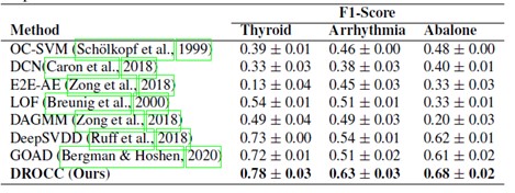
Table 2 shows F1-Score (with standard deviation) for one-vs-all anomaly detection on Thyroid, Arrhythmia, and Abalone datasets from UCI Machine Learning Repository. DROCC outperforms the baselines on all the three datasets by a minimum of 0.07 which is about 11.5% performance increase. Results on One-class Classification with Limited Negatives (OCLN):

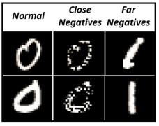
MNIST 0 vs. 1 Classification: We consider an experimental setup on MNIST dataset, where the training data consists of the Digit 0, the normal class, and the Digit 1 as the anomaly. During evaluation, in addition to samples from training distribution, we also have half zeros, which act as challenging OOD points (close negatives). These half zeros are generated by randomly masking 50% of the pixels (Figure 2). BCE performs poorly, with a recall of 54% only at a fixed FPR of 3%. DROCC–OE gives a recall value of 98:16% outperforming DeepSAD by a margin of 7%, which gives a recall value of 90:91%. DROCC–LF provides further improvement with a recall of 99:4% at 3% FPR.

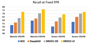
Wake word Detection: Finally, we evaluate DROCC–LF on the practical problem of wake word detection with low FPR against arbitrary OOD negatives. To this end, we identify a keyword, say “Marvin” from the audio commands dataset (Warden, 2018) [8] as the positive class, and the remaining 34 keywords are labeled as the negative class. For training, we sample points uniformly at random from the above-mentioned dataset. However, for evaluation, we sample positives from the train distribution, but negatives contain a few challenging OOD points as well. Sampling challenging negatives itself is a hard task and is the key motivating reason for studying the problem. So, we manually list close-by keywords to Marvin such as: Mar, Vin, Marvelous etc. We then generate audio snippets for these keywords via a speech synthesis tool 2 with a variety of accents. Figure 3 shows that for 3% and 5% FPR settings, DROCC–LF is significantly more accurate than the baselines. For example, with FPR=3%, DROCC–LF is 10% more accurate than the baselines. We repeated the same experiment with the keyword: Seven, and observed a similar trend. In summary, DROCC–LF is able to generalize well against negatives that are “close” to the true positives even when such negatives were not supplied with the training data.
Conclusion and Future Work
We introduced DROCC method for deep anomaly detection. It models normal data points using a low-dimensional manifold, and hence can compare close point via Euclidean distance. Based on this intuition, DROCC’s optimization is formulated as a saddle point problem which is solved via standard gradient descent-ascent algorithm. We then extended DROCC to OCLN problem where the goal is to generalize well against arbitrary negatives, assuming positive class is well sampled and a small number of negative points are also available. Both the methods perform significantly better than strong baselines, in their respective problem settings.
For computational efficiency, we simplified the projection set for both the methods which can perhaps slow down the convergence of the two methods. Designing optimization algorithms that can work with the stricter set is an exciting research direction. Further, we would also like to rigorously analyze DROCC, assuming enough samples from a low-curvature manifold. Finally, as OCLN is an exciting problem that routinely comes up in a variety of real-world applications, we would like to apply DROCC–LF to a few high impact scenarios.
The results of this study showed that DROCC is comparatively better for anomaly detection across many different areas, such as tabular data, images, audio, and time series, when compared to existing state-of-the-art techniques.
It would be interesting to see how the DROCC method performs in situations where the anomaly is very rare, say detecting signals of volacanic explosion from seismic activity data. Such challening anomalous situations will be a test of endurance for this method and can even help advance work in this area.
References
[1]: Golan, I. and El-Yaniv, R. Deep anomaly detection using geometric transformations. In Advances in Neural Information Processing Systems (NeurIPS), 2018.
[2]: Ruff, L., Vandermeulen, R., Goernitz, N., Deecke, L., Siddiqui, S. A., Binder, A., M¨uller, E., and Kloft, M. Deep one-class classification. In International Conference on Machine Learning (ICML), 2018.
[3]: Aggarwal, C. C. Outlier Analysis. Springer Publishing Company, Incorporated, 2nd edition, 2016. ISBN 3319475770.
[4]: Sch¨olkopf, B., Williamson, R., Smola, A., Shawe-Taylor, J., and Platt, J. Support vector method for novelty detection. In Proceedings of the 12th International Conference on Neural Information Processing Systems, 1999.
[5]: Tax, D. M. and Duin, R. P. Support vector data description. Machine Learning, 54(1), 2004.
[6]: Pless, R. and Souvenir, R. A survey of manifold learning for images. IPSJ Transactions on Computer Vision and Applications, 1, 2009.
[7]: Hendrycks, D., Mazeika, M., and Dietterich, T. Deep anomaly detection with outlier exposure. In International Conference on Learning Representations (ICLR), 2019a.
[8]: Warden, P. Speech commands: A dataset for limited vocabulary speech recognition, 2018. URL https: //arxiv.org/abs/1804.03209.
Critiques/Insights
1. It would be interesting to see this implemented in self driving cars, for instance to detect unusual road conditions.
2. Figure 1 shows a good representation on how this model works. However, how can we know that this model is not prone to overfitting? There are many situations where there are valid points that lie outside of the line, especially new data that the model has never see before. An explanation on how this is avoided would be good.
3.In the introduction part, it should first explain what is "one class", and then make detailed application. Moreover, special definition words are used in many places in the text. No detailed explanation was given. In the end, the future application fields of DROCC and the research direction of the group can be explained.
4. The geometry of this technique (classification based on incidence outside of a ball centered at a known point [math]\displaystyle{ x }[/math]) sounds quite similar to K-nearest neighbors. While the authors compared DROCC to single-nearest neighbor classification, choosing a higher K would result in a stronger, more regularized model. It would be interesting to see how DROCC compares to the general KNN classifier