Functional regularisation for continual learning with gaussian processes

Presented by

Meixi Chen

Introduction

Continual Learning (CL) refers to the problem where different tasks are fed to model sequentially, such as training a natural language processing model on different languages over time. A major challenge in CL is model forgets how to solve earlier tasks. This paper proposed a new framework to regularize Continual Learning (CL) so that it doesn't forget previously learned tasks. This method, referred to as functional regularization for Continual Learning, leverages the Gaussian process to construct an approximate posterior belief over the underlying task-specific function. Then the posterior belief is utilized in optimization as a regularizer to prevent the model from completely deviating from the earlier tasks. The estimation of posterior functions is carried out under the framework of approximate Bayesian inference.

Previous Work

There are two types of methods that have been widely used in Continual Learning.

Replay/Rehearsal Methods

This type of methods stores the data or its compressed form from earlier tasks. The stored data is replayed when learning a new task to mitigate forgetting. It can be used for constraining the optimization of new tasks or joint training of both previous and current tasks. However, it has two disadvantages: 1. Deciding which data to store often remains heuristic; 2. Requires a large quantity of stored data to achieve good performance.

Regularization-based Methods

These methods leverage sequential Bayesian inference by putting a prior distribution over the model parameters in a hope to regularize the learning of new tasks. Two important methods are Elastic Weight Consolidation (EWC) and Variational Continual Learning (VCL), both of which make model parameters adaptive to new tasks while regularizing weights by prior knowledge from the earlier tasks. Nonetheless, with long sequences of tasks this might still result in an increased forgetting of earlier tasks.

Comparison between the Proposed Method and Previous Methods

Comparison to regularization-based methods

Similarity: It is also based on approximate Bayesian inference by using a prior distribution that regularizes the model updates.

Difference: It constrains the neural network on the space of functions rather than weights by making use of Gaussian processes (GP).

Comparison to replay/rehearsal methods

Similarity: It also stores data from earlier tasks.

Difference: Instead of storing a subset of data, it stores a set of inducing points, which can be optimized using criteria from GP literature.

Gaussian Process

Definition: A Gaussian process is a collection of random variables, any finite number of which have a joint Gaussian distribution [1].

The Gaussian process is a non-parametric approach as it can be viewed as an infinte-dimensional generalization of multivariate normal distributions. In a very informal sense, it can be thought of as a distribution of continuous functions - this is why we make use of GP to perform optimization in the function space. A Gaussian process over a prediction function [math]\displaystyle{ f(\boldsymbol{x}) }[/math] can be completely specified by its mean function and covariance function (or kernel function), \[\text{Gaussian process: } f(\boldsymbol{x}) \sim \mathcal{GP}(m(\boldsymbol{x}),K(\boldsymbol{x},\boldsymbol{x}'))\] Note that in practice the mean function is typically taken to be 0 because we can always write [math]\displaystyle{ f(\boldsymbol{x})=m(\boldsymbol{x}) + g(\boldsymbol{x}) }[/math] where [math]\displaystyle{ g(\boldsymbol{x}) }[/math] follows a GP with 0 mean. Hence, the GP is characterized by its kernel function.

In fact, we can connect a GP to a multivariate normal (MVN) distribution with 0 mean, which is given by \[\text{Multivariate normal distribution: } \boldsymbol{y} \sim \mathcal{N}(\boldsymbol{0}, \boldsymbol{\Sigma}).\] When we only observe finitely many [math]\displaystyle{ \boldsymbol{x} }[/math], the function's value at these input points is a multivariate normal distribution.

Note: Throughout this summary, [math]\displaystyle{ \mathcal{GP} }[/math] refers the the distribution of functions, and [math]\displaystyle{ \mathcal{N} }[/math] refers to the distribution of finite random variables.

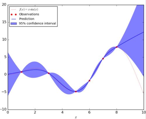
A One-dimensional Example of the Gaussian Process

In the figure below, the red dashed line represents the underlying true function [math]\displaystyle{ f(x) }[/math] and the red dots are the observation taken from this function. The blue solid line indicates the predicted function [math]\displaystyle{ \hat{f}(x) }[/math] given the observations, and the blue shaded area corresponds to the uncertainty of the prediction.

References

[1] Rasmussen, Carl Edward and Williams, Christopher K. I., Gaussian Processes for Machine Learning, The MIT Press, 2006.