Neural ODEs
Introduction
Chen et al. propose a new class of neural networks called neural ordinary differential equations (ODEs) in their 2018 paper under the same title. Neural network models, such as residual or recurrent networks, can be generalized as a set of transformations through hidden states (a.k.a layers) [math]\displaystyle{ \mathbf{h} }[/math], given by the equation
where [math]\displaystyle{ t \in \{0,...,T\} }[/math] and [math]\displaystyle{ \theta_t }[/math] corresponds to the set of parameters or weights in state [math]\displaystyle{ t }[/math]. It is important to note that it has been shown (Lu et al., 2017)(Haber and Ruthotto, 2017)(Ruthotto and Haber, 2018) that the transformation given in Equation 1 can be viewed as an Euler discretization. Given this Euler description, if the number of layers and step size between layers are taken to their limits, then Equation 1 can instead be described continuously in the form of the ODE,
Equation 2 now describes a network where the output layer [math]\displaystyle{ \mathbf{h}(T) }[/math] is generated by solving for the ODE at time [math]\displaystyle{ T }[/math], given the initial value at [math]\displaystyle{ t=0 }[/math], where [math]\displaystyle{ \mathbf{h}(0) }[/math] is the input layer of the network.
With a vast amount of theory and research in the field of solving ODEs numerically, there are a number of benefits to formulating the hidden state dynamics this way. One major advantage is that a continuous description of the network allows for the calculation of [math]\displaystyle{ f }[/math] at arbitrary intervals and locations and is shown in the figure below. The authors also provide a concrete example of this effect in section five with a latent time series model.
The next section on automatic differentiation will describe how utilizing ODE solvers allows for the calculation of gradients of the loss function without the use of backpropagation. A direct result of this is a huge improvement on memory requirements for the model since no intermediate values are stored during forward propagation of the inputs. In section four the authors show that the single-unit bottleneck of normalizing flows can be overcome by constructing a new class of density models that incorporates the neural ODE network formulation.
Reverse-mode Automatic Differentiation of ODE Solutions
Since the depth of a neural ODE network is continuous, there is an inherent challenge to performing backpropagation since you must step back through the steps of the ODE solver. It is noted that one could differentiate along the forward-mode at the price of increased memory and numerical error. Instead, the authors compute the derivatives of the ODE solver with the adjoint sensitivity method (Pontryagin et al., 1962), which alleviates the problems related to memory and accuracy.
The authors provide the example of minimizing a scalar values loss function [math]\displaystyle{ L }[/math] that takes the solution of the ODE solver as its input given by,
where the derivative of this loss function with respect to [math]\displaystyle{ \theta }[/math] is computed by the adjoint method. The adjoint itself is defined as [math]\displaystyle{ \mathbf{a}(t) = \frac{\partial L}{\partial \mathbf{z}(t)} }[/math], which describes the gradient of the loss with respect to the hidden state [math]\displaystyle{ \mathbf{z}(t) }[/math]. By taking the derivative of the adjoint, another ODE arises in the form of,
This provides an easy way to obtain the gradient of [math]\displaystyle{ L }[/math] at [math]\displaystyle{ \mathbf{z}(t_0) }[/math] by solving equation 3, backwards in time from [math]\displaystyle{ \mathbf{z}(t) }[/math]. Finally, the derivative [math]\displaystyle{ dL/d\theta }[/math] can be expressed in terms of the adjoint and the hidden state in the form of the integral,
To obtain efficient calculations of the derivatives in equation 3 and 4, automatic differentiation is used to incur a very small time cost. Subsequently, an efficient algorithm to calculate the gradient of the loss function with only one call to an ODE solver is given in the figure below.
If the loss function has a dependence on intermediate times [math]\displaystyle{ t_i, i \in (0,N) }[/math] then Algorithm 1 can be modified to handle multiple calls to the ODESolve step and is depicted in the figure below.
Please see the appendix for an extended versions of Algorithm 1 and detailed derivations of each equation in this section.
Replacing Residual Networks with ODEs for Supervised Learning
Continuous Normalizing Flows
Section four tackles the implementation of continuous-depth Neural Networks, but to do so, in the first part of section four the authors discuss theoretically how to establish this kind of network through the use of normalizing flows. The authors use a change of variables method presented in other works (Rezende and Mohamed, 2015), (Dinh et al., 2014), to compute the change of a probability distribution if sample points are transformed through a bijective function, [math]\displaystyle{ f }[/math].
Where p(z) is the probability distribution of the samples and [math]\displaystyle{ det\frac{\partial f}{\partial z_0} }[/math] is the determinant of the Jacobian which has a cubic cost in the dimension of z or the number of hidden units in the network. The authors discovered however that transforming the discrete set of hidden layers in the normalizing flow network to continuous transformations simplifies the computations significantly, due primarily to the following theorem:
Theorem 1: (Instantaneous Change of Variables). Let z(t) be a finite continuous random variable with probability p(z(t)) dependent on time. Let dz/dt=f(z(t),t) be a differential equation describing a continuous-in-time transformation of z(t). Assuming that f is uniformly Lipschitz continuous in z and continuous in t, then the change in log probability also follows a differential equation:
The biggest advantage to using this theorem is that the trace function is a linear function, so if the dynamics of the problem, f, is represented by a sum of functions, then so is the log density. This essentially means that you can now compute flow models with only a linear cost with respect to the number of hidden units, [math]\displaystyle{ M }[/math]. In standard normalising flow models, the cost is [math]\displaystyle{ O(M^3) }[/math], so they will generally fit many layers with a single hidden unit in each layer.
Finally the authors use these realizations to construct Continuous Normalizing Flow networks (CNFs) by specifying the parameters of the flow as a function of t, ie, [math]\displaystyle{ f(z(t),t) }[/math]. They also use a gating mechanism for each hidden unit, [math]\displaystyle{ \frac{dz}{dt}=\sum_n \sigma_n(t)f_n(z) }[/math] where [math]\displaystyle{ \sigma_n(t)\in (0,1) }[/math] is a separate neural network which learns when to apply each dynamic [math]\displaystyle{ f_n }[/math].
Section 4.1: implementation
The authors construct two separate types of neural networks to compare against each other, the first is the standard planar Normalizing Flow network (NF) using 64 layers of single hidden units, and the second is their new CNF with 64 hidden units. The NF model is trained over 500,000 iterations using RMSprop, and the CNF network is trained over 10,000 iterations using Adam. The loss function is [math]\displaystyle{ KL(q(x)||p(x)) }[/math] where [math]\displaystyle{ q(x) }[/math] is the flow model and [math]\displaystyle{ p(x) }[/math] is the target probability density.
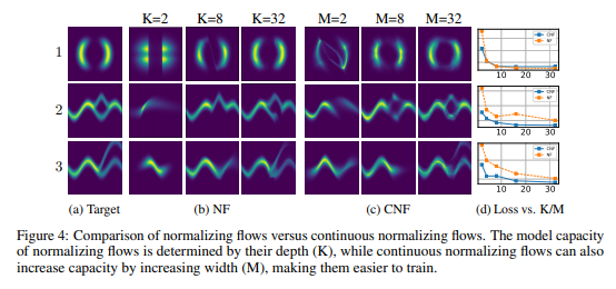
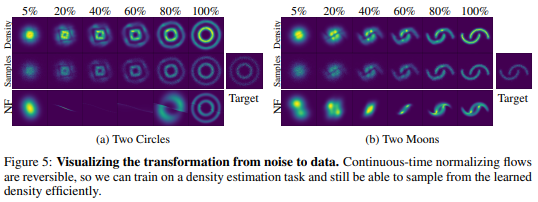
One of the biggest advantages when implementing CNF is that you can train the flow parameters just by performing maximum likelihood estimation on [math]\displaystyle{ log(q(x)) }[/math] given [math]\displaystyle{ p(x) }[/math], where [math]\displaystyle{ q(x) }[/math] is found via the theorem above, and then reversing the CNF to generate random samples from [math]\displaystyle{ q(x) }[/math]. This reversal of the CNF is done with about the same cost of the forward pass which is not able to be done in an NF network. The following two figures demonstrates the ability of CNF to generate more expressive and accurate output data as compared to standard NF networks.
Figure 4 shows clearly that the CNF structure exhibits significantly lower loss functions than NF. In figure 5 both networks were tasked with transforming a standard gaussian distribution into a target distribution, not only was the CNF network more accurate on the two moons target, but also the steps it took along the way are much more intuitive than the output from NF.
A Generative Latent Function Time-Series Model
One of the largest issues at play in terms of Neural ODE networks is the fact that in many instances, data points are either very sparsely distributed, or irregularly-sampled. An example of this is medical records which are only updated when a patient visits a doctor or the hospital. To solve this issue the authors had to create a generative time-series model which would be able to fill in the gaps of missing data. The authors consider each time series as a latent trajectory stemming from the initial local state [math]\displaystyle{ z_{t_0 } }[/math], and determined from a global set of latent parameters. Given a set of observation times and initial state, the generative model constructs points via the following sample procedure:
[math]\displaystyle{ z_{t_0}∼p(z_{t_0}) }[/math]
[math]\displaystyle{ z_{t_1},z_{t_2},\dots,z_{t_N}=ODESolve(z_{t_0},f,θ_f,t_0,...,t_N) }[/math]
each [math]\displaystyle{ x_{t_i}∼p(x│z_{t_i},θ_x) }[/math]
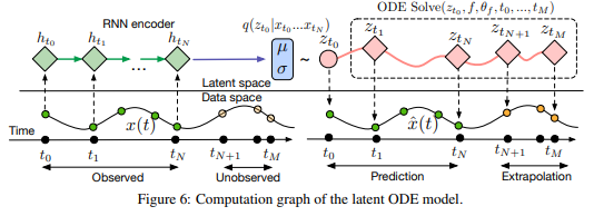
[math]\displaystyle{ f }[/math] is a function which outputs the gradient [math]\displaystyle{ \frac{\partial z(t)}{\partial t}=f(z(t),θ_f) }[/math] which is parameterized via a neural net. In order to train this latent variable model, the authors had to first encode their given data and observation times using an RNN encoder, construct the new points using the trained parameters, then decode the points back into the original space. The following figure describes this process:
Another variable which could affect the latent state of a time-series model is how often an event actually occurs. The authors solved this by parameterizing the rate of events in terms of a Poisson process. They described the set of independent observation times in an interval [math]\displaystyle{ \left[t_{start},t_{end}\right] }[/math] as:
[math]\displaystyle{ log(p(t_1,t_2,\dots,t_N ))=\sum_{i=1}^Nlog(\lambda(z(t_i)))-\int_{t_{start}}^{t_{end}}λ(z(t))dt }[/math]
where [math]\displaystyle{ \lambda(*) }[/math] is parameterized via another neural network.
Section 5.1: Implementation
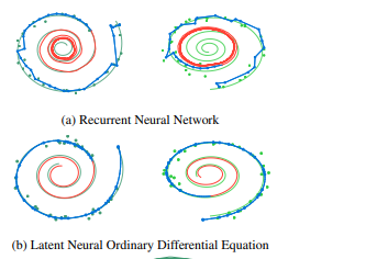
To test the effectiveness of the Latent time-series ODE model (LODE), they fit the encoder with 25 hidden units, parametrize function f with a one-layer 20 hidden unit network, and the decoder as another neural network with 20 hidden units. They compare this against a standard recurrent neural net (RNN) with 25 hidden units trained to minimize gaussian log-likelihood. The authors tested both of these network systems on a dataset of 2-dimensional spirals which either rotated clockwise or counter-clockwise, and sampled the positions of each spiral at 100 equally spaced time steps. They can then simulate irregularly timed data by taking random amounts of points without replacement from each spiral. The next two figures show the outcome of these experiments:
In the figure on the right the blue lines represent the test data learned curves and the red lines represent the extrapolated curves predicted by each model. It is noted that the LODE performs significantly better than the standard RNN model, especially on smaller sets of datapoints.
Scope and Limitations
Section 6 mainly discusses the scope and limitations of the paper. Firstly while “batching” the training data is a useful step in standard neural nets, and can still be applied here by combining the ODEs associated with each batch, the authors found that that controlling error in this case may increase the number of calculations required. In practice however the number of calculations did not increase significantly.
So long as the model proposed in this paper uses finite weights and Lipschitz nonlinearities, then Picard’s existence theorem (Coddington and Levinson, 1955) applies, guaranteeing the solution to the IVP exists and is unique.
In controlling the amount of error in the model, the authors were only able to reduce tolerances to approximately [math]\displaystyle{ 1e-3 }[/math] and [math]\displaystyle{ 1e-5 }[/math] in classification and density estimation respectively without also degrading the computational performance.
The authors believe that reconstructing state trajectories by running the dynamics backwards can introduce extra numerical error. They address a possible solution to this problem by checkpointing certain time steps and storing intermediate values of z on the forward pass. Then while reconstructing, you do each part individually between checkpoints. The authors acknowledged that they informally checked the validity of this method since they don’t consider it a practical problem.
Conclusions and Critiques
Link to Appendices of Paper
https://arxiv.org/pdf/1806.07366.pdf


