stat841

Classfication-2009.9.30

Classification

With the rising fields of data-mining, bioinformatics, machine learning and so on, classification has becomes a fast developing topic. In the age of information, vast amount of data is generated constantly, and the goal of classification is to learn from data. Potential application areas include handwritten post codes recognition, medical diagnosis, face recognition, human language processing and so on.

In classification we attempt to approximate a function [math]\displaystyle{ \,h }[/math], by using a training data set, that will then be able to accurately classify new data inputs.

Given [math]\displaystyle{ \mathcal{X} \subset \mathbb{R}^{d} }[/math], a subset of the [math]\displaystyle{ D }[/math]-dimensional real vectors and [math]\displaystyle{ \mathcal{Y} }[/math], a finite set of labels, We try to determine a 'classification rule' [math]\displaystyle{ \,h }[/math] such that,

[math]\displaystyle{ \,h: \mathcal{X} \mapsto \mathcal{Y} }[/math]

We use [math]\displaystyle{ \,n }[/math] ordered pairs of training data, [math]\displaystyle{ \,\{(X_{1},Y_{1}), (X_{2},Y_{2}), \dots , (X_{n},Y_{n})\} }[/math] where [math]\displaystyle{ \,X_{i} \in \mathcal{X} }[/math],[math]\displaystyle{ \,Y_{i} \in \mathcal{Y} }[/math], to approximate [math]\displaystyle{ \,h }[/math].

Thus, given a new input, [math]\displaystyle{ \,X \in \mathcal{X} }[/math] by using the classification rule we can predict a corresponding [math]\displaystyle{ \,\hat{Y}=h(X) }[/math].

Example Suppose we wish to classify fruits into apples and oranges by considering certain features of the fruit, e.g, color, diameter, and weight.
Let [math]\displaystyle{ \mathcal{X}= (\mathrm{colour}, \mathrm{diameter}, \mathrm{weight}) }[/math] and [math]\displaystyle{ \mathcal{Y}=\{\mathrm{apple}, \mathrm{orange}\} }[/math]. The goal is to find a classification rule such that when a new fruit [math]\displaystyle{ \,X }[/math] is presented based on its features, [math]\displaystyle{ (\,X_{\mathrm{color}}, X_{\mathrm{diameter}}, X{_\mathrm{weight}}) }[/math], our classification rule [math]\displaystyle{ \,h }[/math] can classify it as either an apple or an orange, i.e., [math]\displaystyle{ \,h(X_{\mathrm{color}}, X_{\mathrm{diameter}}, X_{\mathrm{weight}}) }[/math] be the fruit type of [math]\displaystyle{ \,X }[/math].

Error rate

'True error rate' of a classifier(h) is defined as the probability that [math]\displaystyle{ \,h }[/math] does not correctly classify the points of [math]\displaystyle{ \,\mathcal{X} }[/math], i.e.,

[math]\displaystyle{ \, L(h)=P(h(X) \neq Y) }[/math]

'Empirical error rate(training error rate)' of a classifier(h) is defined as the frequency that [math]\displaystyle{ \,h }[/math] does not correctly classify the points in the training set, i.e.,

[math]\displaystyle{ \, L_{h}= \frac{1}{n} \sum_{i=1}^{n} I(h(X_{i}) \neq Y_{i}) }[/math], where [math]\displaystyle{ \,I }[/math] is an indicator that [math]\displaystyle{ \, I= \left\{\begin{matrix} 1 & h(X_i) \neq Y_i \\ 0 & h(X_i)=Y_i \end{matrix}\right. }[/math].

Bayes Classifier

The principle of Bayes Classifier is to calculate posteriori probability of given object from its priors probability via Bayes formula, and then choose the class with biggest posteriori probability as the one what the object affiliated with. Intuitively speaking to classify [math]\displaystyle{ \,x\in \mathcal{X} }[/math] we find [math]\displaystyle{ y \in \mathcal{Y} }[/math] such that [math]\displaystyle{ \,P(Y=y|X=x) }[/math] is maximum over all the members of [math]\displaystyle{ \mathcal{Y} }[/math].

Mathematically, for [math]\displaystyle{ \,k }[/math] classes and given object [math]\displaystyle{ \,X=x }[/math], we are going to find out [math]\displaystyle{ \,y_{i}\in \mathcal{Y} }[/math] which maximizes [math]\displaystyle{ \,P(Y=y_i|X=x) }[/math], and classify [math]\displaystyle{ \,X }[/math] into class [math]\displaystyle{ \,y_{i} }[/math]. In order to calculate the value of [math]\displaystyle{ \,P(Y=y_{i}|X=x) }[/math], we use the Bayes formula

[math]\displaystyle{ \begin{align} P(Y=y|X=x) &= \frac{P(X=x|Y=y)P(Y=y)}{P(X=x)} \\ &=\frac{P(X=x|Y=y)P(Y=y)}{\Sigma_{\forall y \in \mathcal{Y}}P(X=x|Y=y)P(Y=y)} \end{align} }[/math]

where [math]\displaystyle{ \,P(Y=y|X=x) }[/math] is referred to as the posteriori probability, [math]\displaystyle{ \,P(Y=y) }[/math] as the priors probability, [math]\displaystyle{ \,P(X=x|Y=y) }[/math] as the likelihood, and [math]\displaystyle{ \,P(X=x) }[/math] as the evidence.

For the special case that [math]\displaystyle{ \,Y }[/math] has only two possible values, that is, [math]\displaystyle{ \, \mathcal{Y}=\{0, 1\} }[/math]. Consider the probability that [math]\displaystyle{ \,r(X)=P\{Y=1|X=x\} }[/math]. Given [math]\displaystyle{ \,X=x }[/math], By Bayes formula, we have

[math]\displaystyle{ \begin{align} r(X)&=P(Y=1|X=x) \\ &=\frac{P(X=x|Y=1)P(Y=1)}{P(X=x)}\\ &=\frac{P(X=x|Y=1)P(Y=1)}{P(X=x|Y=1)P(Y=1)+P(X=x|Y=0)P(Y=0)} \end{align} }[/math]

Definition:

The Bayes classification rule [math]\displaystyle{ \,h }[/math] is

[math]\displaystyle{ \, h(X)= \left\{\begin{matrix} 1 & r(x)\gt \frac{1}{2} \\ 0 & \mathrm{otherwise} \end{matrix}\right. }[/math]

Bayes classification rule optimality Theorem: The Bayes rule is optimal in true error rate, that is for any other classification rule [math]\displaystyle{ \, \overline{h} }[/math], we have [math]\displaystyle{ \,L(\overline{h}) \le L(h) }[/math]. Intuitively speaking this theorem is saying we cannot do better than classifying [math]\displaystyle{ \,x\in \mathcal{X} }[/math] to [math]\displaystyle{ \,y }[/math] when the probability of being of type [math]\displaystyle{ \,y }[/math] for [math]\displaystyle{ \,x }[/math] is more than probability of being any other type.

Definition:

The set [math]\displaystyle{ \,D(h)=\{x: P(Y=1|X=x)=P(Y=0|X=x)\} }[/math] is called the decision boundary.

Example:
We’re going to predict if a particular student will pass STAT441/841. We have data on past student performance. For each student we know: If student’s GPA > 3.0 (G) If student had a strong math background (M) If student is a hard worker (H) If student passed or failed course

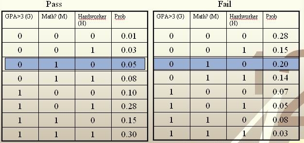
[math]\displaystyle{ \, \mathcal{Y}= \{ 0,1 \} }[/math], where 1 refers to pass and 0 refers to fail. Assume that [math]\displaystyle{ \,P(Y=1)=P(Y=0)=0.5 }[/math]
For a new student comes along with values [math]\displaystyle{ \,G=0, M=1, H=0 }[/math], we calculate [math]\displaystyle{ \,r(X)=P(Y=1|X=(0,1,0)) }[/math] as

[math]\displaystyle{ \,r(X)=P(Y=1|X=(0,1,0))=\frac{P(X=(0,1,0)|Y=1)P(Y=1)}{P(X=(0,1,0)|Y=1)P(Y=1)+P(X=(0,1,0)|Y=0)P(Y=0)}=\frac{0.025}{0.125}=0.2\lt \frac{1}{2} }[/math]
Thus, we classify the new student into class 0, namely, we predict him to fail in this course.

Notice: Although the Bayes rule is optimal, we still need other methods, and the reason for the fact is that in the Bayes equation discussed before, it is generally impossible for us to know the [math]\displaystyle{ \,P(Y=1) }[/math], and [math]\displaystyle{ \,P(X=x|Y=1) }[/math] and ultimately calculate the value of [math]\displaystyle{ \,r(X) }[/math], which makes Bayes rule inconvenient in practice.

Currently, there are four primary classifier based on Bayes Classifier: Naive Bayes classifier[1], TAN, BAN and GBN.
useful link:Decision Theory, Bayes Classifier

Bayes VS Frequentist

Intuitively, to solve a two-class problem, we may have the following two approaches:

1) If [math]\displaystyle{ \,P(Y=1|X=x)\gt P(Y=0|X=x) }[/math], then [math]\displaystyle{ \,h(x)=1 }[/math], otherwise [math]\displaystyle{ \,h(x)=0 }[/math].

2) If [math]\displaystyle{ \,P(X=x|Y=1)\gt P(X=x|Y=0) }[/math], then [math]\displaystyle{ \,h(x)=1 }[/math], otherwise [math]\displaystyle{ \,h(x)=0 }[/math].

One obvious difference between these two methods is that the first one considers probability as changing based on observation while the second one considers probablity as objective existance. Actually, they represent two different schools in statistics.

During the history of statistics, there are two major classification methods : Bayes and frequentist. The two methods represent two different ways of thoughts and hold different view to define probability. The followings are the main differences between Bayes and Frequentist.

Frequentist

1. Probability is objective.
2. Data is a repeatable random sample(there is a frequency).
3. Parameters are fixed and unknown constant.
4. Not applicable to single event. For example, a frequentist cannot predict the weather of tomorrow because tomorrow is only one unique event, and cannot be referred to a frequency in a lot of samples.

Bayes

1. Probability is subjective.
2. Data are fixed.
3. Parameters are unknown and random variables that have a given distribution and other probability statements can be made about them.
4. Can be applied to single events based on degree of confidence or beliefs. For example, Bayesian can predict tomorrow's weather, such as having the probability of [math]\displaystyle{ \,50% }[/math] of rain.

Example

Suppose there is a man named Jack. In bayes method, at first, one can see this man (object), and then judge whether his name is Jack (label). On the other hand, in Frequentist method, one doesn’t see the man (object), but can see the photos (label) of this man to judge whether he is Jack.

Linear and Quadratic Discriminant Analysis - October 2,2009

Introduction

Notation

Let us first introduce some new notation for the following sections.

Recall that in the discussion of the Bayes Classifier, we introduced Bayes Formula:

[math]\displaystyle{ \begin{align} P(Y=y|X=x) &=\frac{P(X=x|Y=y)P(Y=y)}{\Sigma_{\forall y \in \mathcal{Y}}P(X=x|Y=y)P(Y=y)} \end{align} }[/math]

We will use new labels for the following equivalent formula:

[math]\displaystyle{ \begin{align} P(Y=k|X=x) &=\frac{f_k(x)\pi_k}{\Sigma_kf_k(x)\pi_k} \end{align} }[/math]

• [math]\displaystyle{ \,f_k }[/math] is called the class conditional density; also referred to previously as the likelihood function. Essentially, this is the function that allows us to reason about a parameter given a certain outcome.
• [math]\displaystyle{ \,\pi_k }[/math] is called the prior probability. This is a probability distribution that represents what we know (or believe we know) about a population.
• [math]\displaystyle{ \,\Sigma_k }[/math] is the sum with respect to all [math]\displaystyle{ \,k }[/math] classes.

Approaches

Representing the optima method, Bayes classifier cannot be used in most practical situations though, since usually the prior probability is unknown. Fortunately, other methods of classification have evolved. These methods fall into three general categories.

1. Choose classifiers, find [math]\displaystyle{ \,h^* \epsilon H }[/math], minimize some estimate of [math]\displaystyle{ \,L(H) }[/math].
2. Regression
3. Density estimation, estimate [math]\displaystyle{ P(X = x | Y = 0) }[/math] and [math]\displaystyle{ P(X = x | Y = 1) }[/math]

The third approach, in this form, is not popular because density estimation doesn't work very well with dimension greater than 2. Linear Discriminate Analysis and Quadratic Discriminate Analysis are examples of the third approach, density estimation.

LDA

Motivation

The Bayes classifier is optimal. Unfortunately, the prior and conditional density of most data is not known. Some estimation of these should be made if we want to classify some data.

The simplest way to achieve this is to assume that all the class densities are approximately a multivariate normal distribution, find the parameters of each such distribution, and use them to calculate the conditional density and prior for unknown points, thus approximating the Bayesian classifier to choose the most likely class. In addition, if the covariance of each class density is assumed to be the same, the number of unknown parameters is reduced and the model is easy to fit and use, as seen later.

History

The name Linear Discriminant Analysis comes from the fact that these simplifications produce a linear model, which is used to discriminate between classes. In many cases, this simple model is sufficient to provide a near optimal classification - for example, the Z-Score credit risk model, designed by Edward Altman in 1968, which is essentially a weighted LDA, revisited in 2000, has shown an 85-90% success rate predicting bankruptcy, and is still in use today.

Definition

To perform LDA we make two assumptions.

1. The clusters belonging to all classes each follow a multivariate normal distribution.
   [math]\displaystyle{ x \in \mathbb{R}^d }[/math] [math]\displaystyle{ f_k(x)=\frac{1}{ (2\pi)^{d/2}|\Sigma_k|^{1/2} }\exp\left( -\frac{1}{2} [x - \mu_k]^\top \Sigma_k^{-1} [x - \mu_k] \right) }[/math]
2. Each cluster has the same variance [math]\displaystyle{ \,\Sigma }[/math] equal to the mean variance of [math]\displaystyle{ \Sigma_k \forall k }[/math].

We wish to solve for the boundary where the error rates for classifying a point are equal, where one side of the boundary gives a lower error rate for one class and the other side gives a lower error rate for the other class.

So we solve [math]\displaystyle{ \,r_k(x)=r_l(x) }[/math] for all the pairwise combinations of classes.

[math]\displaystyle{ \,\Rightarrow Pr(Y=k|X=x)=Pr(Y=l|X=x) }[/math]

[math]\displaystyle{ \,\Rightarrow \frac{Pr(X=x|Y=k)Pr(Y=k)}{Pr(X=x)}=\frac{Pr(X=x|Y=l)Pr(Y=l)}{Pr(X=x)} }[/math] using Bayes' Theorem

[math]\displaystyle{ \,\Rightarrow Pr(X=x|Y=k)Pr(Y=k)=Pr(X=x|Y=l)Pr(Y=l) }[/math] by canceling denominators

[math]\displaystyle{ \,\Rightarrow f_k(x)\pi_k=f_l(x)\pi_l }[/math]

[math]\displaystyle{ \,\Rightarrow \frac{1}{ (2\pi)^{d/2}|\Sigma|^{1/2} }\exp\left( -\frac{1}{2} [x - \mu_k]^\top \Sigma^{-1} [x - \mu_k] \right)\pi_k=\frac{1}{ (2\pi)^{d/2}|\Sigma|^{1/2} }\exp\left( -\frac{1}{2} [x - \mu_l]^\top \Sigma^{-1} [x - \mu_l] \right)\pi_l }[/math]

[math]\displaystyle{ \,\Rightarrow \exp\left( -\frac{1}{2} [x - \mu_k]^\top \Sigma^{-1} [x - \mu_k] \right)\pi_k=\exp\left( -\frac{1}{2} [x - \mu_l]^\top \Sigma^{-1} [x - \mu_l] \right)\pi_l }[/math] Since both [math]\displaystyle{ \Sigma }[/math] are equal based on the assumptions specific to LDA.

[math]\displaystyle{ \,\Rightarrow -\frac{1}{2} [x - \mu_k]^\top \Sigma^{-1} [x - \mu_k] + \log(\pi_k)=-\frac{1}{2} [x - \mu_l]^\top \Sigma^{-1} [x - \mu_l] +\log(\pi_l) }[/math] taking the log of both sides.

[math]\displaystyle{ \,\Rightarrow \log(\frac{\pi_k}{\pi_l})-\frac{1}{2}\left( x^\top\Sigma^{-1}x + \mu_k^\top\Sigma^{-1}\mu_k - 2x^\top\Sigma^{-1}\mu_k - x^\top\Sigma^{-1}x - \mu_l^\top\Sigma^{-1}\mu_l + 2x^\top\Sigma^{-1}\mu_l \right)=0 }[/math] by expanding out

[math]\displaystyle{ \,\Rightarrow \log(\frac{\pi_k}{\pi_l})-\frac{1}{2}\left( \mu_k^\top\Sigma^{-1}\mu_k-\mu_l^\top\Sigma^{-1}\mu_l - 2x^\top\Sigma^{-1}(\mu_k-\mu_l) \right)=0 }[/math] after canceling out like terms and factoring.

We can see that this is a linear function in x with general form ax+b=0.

Actually, this linear log function shows that the decision boundary between class [math]\displaystyle{ k }[/math] and class [math]\displaystyle{ l }[/math], i.e. [math]\displaystyle{ Pr(G=k|X=x)=Pr(G=l|X=x) }[/math], is linear in [math]\displaystyle{ x }[/math]. Given any pair of classes, decision boundaries are always linear. In [math]\displaystyle{ p }[/math] dimensions, we separate regions by hyperplanes.

In the special case where the number of samples from each class are equal ([math]\displaystyle{ \,\pi_k=\pi_l }[/math]), the boundary surface or line lies halfway between [math]\displaystyle{ \,\mu_l }[/math] and [math]\displaystyle{ \,\mu_k }[/math]

QDA

The concept is the same idea of finding a boundary where the error rate for classification between classes are equal, except the assumption that each cluster has the same variance [math]\displaystyle{ \,\Sigma }[/math] equal to the mean variance of [math]\displaystyle{ \Sigma_k \forall k }[/math] is removed.

Following along from where QDA diverges from LDA.

[math]\displaystyle{ \,f_k(x)\pi_k=f_l(x)\pi_l }[/math]

[math]\displaystyle{ \,\Rightarrow \frac{1}{ (2\pi)^{d/2}|\Sigma_k|^{1/2} }\exp\left( -\frac{1}{2} [x - \mu_k]^\top \Sigma_k^{-1} [x - \mu_k] \right)\pi_k=\frac{1}{ (2\pi)^{d/2}|\Sigma_l|^{1/2} }\exp\left( -\frac{1}{2} [x - \mu_l]^\top \Sigma_l^{-1} [x - \mu_l] \right)\pi_l }[/math]

[math]\displaystyle{ \,\Rightarrow \frac{1}{|\Sigma_k|^{1/2} }\exp\left( -\frac{1}{2} [x - \mu_k]^\top \Sigma_k^{-1} [x - \mu_k] \right)\pi_k=\frac{1}{|\Sigma_l|^{1/2} }\exp\left( -\frac{1}{2} [x - \mu_l]^\top \Sigma_l^{-1} [x - \mu_l] \right)\pi_l }[/math] by cancellation

[math]\displaystyle{ \,\Rightarrow -\frac{1}{2}\log(|\Sigma_k|)-\frac{1}{2} [x - \mu_k]^\top \Sigma_k^{-1} [x - \mu_k]+\log(\pi_k)=-\frac{1}{2}\log(|\Sigma_l|)-\frac{1}{2} [x - \mu_l]^\top \Sigma_l^{-1} [x - \mu_l]+\log(\pi_l) }[/math] by taking the log of both sides

[math]\displaystyle{ \,\Rightarrow \log(\frac{\pi_k}{\pi_l})-\frac{1}{2}\log(\frac{|\Sigma_k|}{|\Sigma_l|})-\frac{1}{2}\left( x^\top\Sigma_k^{-1}x + \mu_k^\top\Sigma_k^{-1}\mu_k - 2x^\top\Sigma_k^{-1}\mu_k - x^\top\Sigma_l^{-1}x - \mu_l^\top\Sigma_l^{-1}\mu_l + 2x^\top\Sigma_l^{-1}\mu_l \right)=0 }[/math] by expanding out

[math]\displaystyle{ \,\Rightarrow \log(\frac{\pi_k}{\pi_l})-\frac{1}{2}\log(\frac{|\Sigma_k|}{|\Sigma_l|})-\frac{1}{2}\left( x^\top(\Sigma_k^{-1}-\Sigma_l^{-1})x + \mu_k^\top\Sigma_k^{-1}\mu_k - \mu_l^\top\Sigma_l^{-1}\mu_l - 2x^\top(\Sigma_k^{-1}\mu_k-\Sigma_l^{-1}\mu_l) \right)=0 }[/math] this time there are no cancellations, so we can only factor

The final result is a quadratic equation specifying a curved boundary between classes with general form ax²+bx+c=0.

Linear and Quadratic Discriminant Analysis cont'd - October 5, 2009

Summarizing LDA and QDA

We can summarize what we have learned on LDA and QDA so far into the following theorem.

Theorem:

Suppose that [math]\displaystyle{ \,Y \in \{1,\dots,k\} }[/math], if [math]\displaystyle{ \,f_k(x) = Pr(X=x|Y=y) }[/math] is Gaussian, the Bayes Classifier rule is:

[math]\displaystyle{ \,h(X) = \arg\max_{k} \delta_k(x) }[/math]

where

[math]\displaystyle{ \,\delta_k = - \frac{1}{2}log(|\Sigma_k|) - \frac{1}{2}(x-\mu_k)^\top\Sigma_k^{-1}(x-\mu_k) + log (\pi_k) }[/math] (quadratic)

• Note The decision boundary between classes [math]\displaystyle{ k }[/math] and [math]\displaystyle{ l }[/math] is quadratic in [math]\displaystyle{ x }[/math].

If the covariance of the Gaussians are the same, this becomes:

[math]\displaystyle{ \,\delta_k = x^\top\Sigma^{-1}\mu_k - \frac{1}{2}\mu_k^\top\Sigma^{-1}\mu_k + log (\pi_k) }[/math] (linear)

• Note [math]\displaystyle{ \,\arg\max_{k} \delta_k(x) }[/math]returns the set of k for which [math]\displaystyle{ \,\delta_k(x) }[/math] attains its largest value.

In practice

We need to estimate the prior, so in order to do this, we use the sample estimates of [math]\displaystyle{ \,\pi,\mu_k,\Sigma_k }[/math] in place of the true values, i.e.

File:estimation.png

Estimation of the probability of belonging to either class k or l

[math]\displaystyle{ \,\hat{\pi_k} = \hat{Pr}(y=k) = \frac{n_k}{n} }[/math]

[math]\displaystyle{ \,\hat{\mu_k} = \frac{1}{n_k}\sum_{i:y_i=k}x_i }[/math]

[math]\displaystyle{ \,\hat{\Sigma_k} = \frac{1}{n_k}\sum_{i:y_i=k}(x_i-\hat{\mu_k})(x_i-\hat{\mu_k})^\top }[/math]

In the case where we have a common covariance matrix, we get the ML estimate to be

[math]\displaystyle{ \,\Sigma=\frac{\sum_{r=1}^{k}(n_r\Sigma_r)}{\sum_{l=1}^{k}(n_l)} }[/math]

Computation

Case 1: (Example) [math]\displaystyle{ \, \Sigma_k = I }[/math]

This means that the data is distributed symmetrically around the center [math]\displaystyle{ \mu }[/math], i.e. the isocontours are all circles.

We have:

[math]\displaystyle{ \,\delta_k = - \frac{1}{2}log(|I|) - \frac{1}{2}(x-\mu_k)^\top I(x-\mu_k) + log (\pi_k) }[/math]

We see that the first term in the above equation, [math]\displaystyle{ \,\frac{1}{2}log(|I|) }[/math], is zero. The second term contains [math]\displaystyle{ \, (x-\mu_k)^\top I(x-\mu_k) = (x-\mu_k)^\top(x-\mu_k) }[/math], which is the squared Euclidean distance between [math]\displaystyle{ \,x }[/math] and [math]\displaystyle{ \,\mu_k }[/math]. Therefore we can find the distance between a point and each center and adjust it with the log of the prior, [math]\displaystyle{ \,log(\pi_k) }[/math]. The class that has the minimum distance will maximise [math]\displaystyle{ \,\delta_k }[/math]. According to the theorem, we can then classify the point to a specific class [math]\displaystyle{ \,k }[/math]. In addition, [math]\displaystyle{ \, \Sigma_k = I }[/math] implies that our data is spherical.

Case 2: (General Case) [math]\displaystyle{ \, \Sigma_k \ne I }[/math]

We can decompose this as:

[math]\displaystyle{ \, \Sigma_k = USV^\top = USU^\top }[/math] (since if [math]\displaystyle{ \, U = XX^\top }[/math] and [math]\displaystyle{ \, V=X^\top X }[/math] , if [math]\displaystyle{ \, X }[/math] is symmetric, [math]\displaystyle{ \, U=V }[/math] , and here [math]\displaystyle{ \, \Sigma }[/math] is symmetric)

and the inverse of [math]\displaystyle{ \,\Sigma_k }[/math] is

[math]\displaystyle{ \, \Sigma_k^{-1} = (USU^\top)^{-1} = (U^\top)^{-1}S^{-1}U^{-1} = US^{-1}U^\top }[/math] (since [math]\displaystyle{ \,U }[/math] is orthonormal)

So from the formula for [math]\displaystyle{ \,\delta_k }[/math], the second term is

[math]\displaystyle{ \, (x-\mu_k)^\top\Sigma_k^{-1}(x-\mu_k) }[/math]

[math]\displaystyle{ \, = (x-\mu_k)^\top US^{-1}U^T(x-\mu_k) }[/math]

[math]\displaystyle{ \, = (U^\top x-U^\top\mu_k)^\top S^{-1}(U^\top x-U^\top \mu_k) }[/math]

[math]\displaystyle{ \, = (U^\top x-U^\top\mu_k)^\top S^{-\frac{1}{2}}S^{-\frac{1}{2}}(U^\top x-U^\top\mu_k) }[/math]

[math]\displaystyle{ \, = (S^{-\frac{1}{2}}U^\top x-S^{-\frac{1}{2}}U^\top\mu_k)^\top I(S^{-\frac{1}{2}}U^\top x-S^{-\frac{1}{2}}U^\top \mu_k) }[/math]

[math]\displaystyle{ \, = (S^{-\frac{1}{2}}U^\top x-S^{-\frac{1}{2}}U^\top\mu_k)^\top(S^{-\frac{1}{2}}U^\top x-S^{-\frac{1}{2}}U^\top \mu_k) }[/math]

where we have the Euclidean distance between [math]\displaystyle{ \, S^{-\frac{1}{2}}U^\top x }[/math] and [math]\displaystyle{ \, S^{-\frac{1}{2}}U^\top\mu_k }[/math].

A transformation of all the data points can be done from [math]\displaystyle{ \,x }[/math] to [math]\displaystyle{ \,x^* }[/math] where [math]\displaystyle{ \, x^* \leftarrow S^{-\frac{1}{2}}U^\top x }[/math].

It is now possible to do classification with [math]\displaystyle{ \,x^* }[/math], treating it as in Case 1 above.

Note that when we have multiple classes, they must all have the same transformation, else, ahead of time we would have to assume a data point belongs to one class or the other. All classes therefore need to have the same shape for classification to be applicable using this method. So this method works for LDA.

If the classes have different shapes, in another word, have different covariance [math]\displaystyle{ \,\Sigma_k }[/math], can we use the same method to transform all data points [math]\displaystyle{ \,x }[/math] to [math]\displaystyle{ \,x^* }[/math]?

The answer is NO. Consider that you have two classes with different shapes, then consider transforming them to the same shape. Given a data point, justify which class this point belongs to. The question is, which transformation can you use? For example, if you use the transformation of class A, then you have assumed that this data point belongs to class A.

The Number of Parameters in LDA and QDA

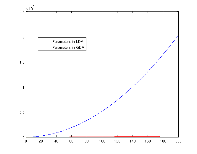
Both LDA and QDA require us to estimate parameters. The more estimation we have to do, the less robust our classification algorithm will be.

LDA: Since we just need to compare the differences between one given class and remaining [math]\displaystyle{ \,K-1 }[/math] classes, totally, there are [math]\displaystyle{ \,K-1 }[/math] differences. For each of them, [math]\displaystyle{ \,a^{T}x+b }[/math] requires [math]\displaystyle{ \,d+1 }[/math] parameters. Therefore, there are [math]\displaystyle{ \,(K-1)\times(d+1) }[/math] parameters.

QDA: For each of the differences, [math]\displaystyle{ \,x^{T}ax + b^{T}x + c }[/math] requires [math]\displaystyle{ \frac{1}{2}(d+1)\times d + d + 1 = \frac{d(d+3)}{2}+1 }[/math] parameters. Therefore, there are [math]\displaystyle{ (K-1)(\frac{d(d+3)}{2}+1) }[/math] parameters.

A plot of the number of parameters that must be estimated, in terms of (K-1). The x-axis represents the number of dimensions in the data. As is easy to see, QDA is far less robust than LDA for high-dimensional data sets.

LDA and QDA in Matlab - October 7, 2009

We have examined the theory behind Linear Discriminant Analysis (LDA) and Quadratic Discriminant Analysis (QDA) above; how do we use these algorithms in practice? Matlab offers us a function called classify that allows us to perform LDA and QDA quickly and easily.

In class, we were shown an example of using LDA and QDA on the 2_3 data that is used in the first assignment. The code below reproduces that example, slightly modified, and explains each step.

>> load 2_3;
>> [U, sample] = princomp(X');
>> sample = sample(:,1:2);

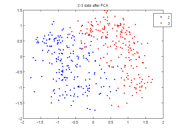
First, we do principal component analysis (PCA) on the 2_3 data to reduce the dimensionality of the original data from 64 dimensions to 2. Doing this makes it much easier to visualize the results of the LDA and QDA algorithms.

>> plot (sample(1:200,1), sample(1:200,2), '.');
>> hold on;
>> plot (sample(201:400,1), sample(201:400,2), 'r.');

Recall that in the 2_3 data, the first 200 elements are images of the number two handwritten and the last 200 elements are images of the number three handwritten. This code sets up a plot of the data such that the points that represent a 2 are blue, while the points that represent a 3 are red.

See title and legend for information on adding the title and legend.

Before using classify we can set up a vector that contains the actual labels for our data, to train the classification algorithm. If we don't know the labels for the data, then the element in the group vector should be an empty string or NaN. (See grouping data for more information.)

>> group = ones(400,1);
>> group(201:400) = 2;

We can now classify our data.

>> [class, error, POSTERIOR, logp, coeff] = classify(sample, sample, group, 'linear');

The full details of this line can be examined in the Matlab help file linked above. What we care about are class, which contains the labels that the algorithm thinks that each data point belongs to, and coeff, which contains information about the line that algorithm created to separate the data into each class.

We can see the efficacy of the algorithm by comparing class to group.

>> sum (class==group)
ans =
   369

This compares the value in class to the value in group. The answer of 369 tells us that the algorithm correctly determined the class of the point 369 times, out of a possible 400 data points. This gives us an empirical error rate of 0.0775.

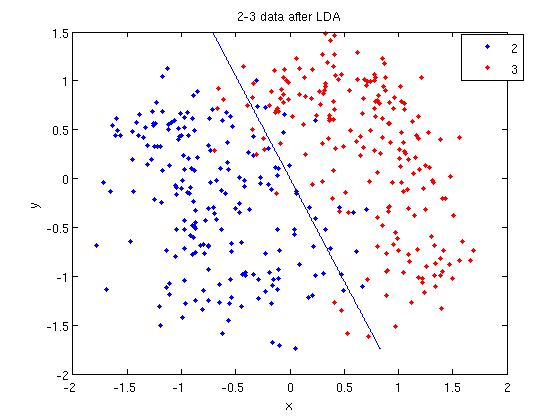
We can see the line produced by LDA using coeff.

>> k = coeff(1,2).const;
>> l = coeff(1,2).linear;
>> f = sprintf('0 = %g+%g*x+%g*y', k, l(1), l(2));
>> ezplot(f, [min(sample(:,1)), max(sample(:,1)), min(sample(:,2)), max(sample(:,2))]);

Those familiar with the programming language C will find the sprintf line refreshingly familiar; those with no exposure to C are directed to Matlab's sprintf page. Essentially, this code sets up the equation of the line in the form 0 = a + bx + cy. We then use the ezplot function to plot the line.

The 2-3 data after LDA is performed. The line shows where the two classes are split.

Let's perform the same steps, except this time using QDA. The main difference with QDA is a slightly different call to classify, and a more complicated procedure to plot the line.

>> [class, error, POSTERIOR, logp, coeff] = classify(sample, sample, group, 'quadratic');
>> sum (class==group)
ans =
   371
>> k = coeff(1,2).const;
>> l = coeff(1,2).linear;
>> q = coeff(1,2).quadratic;
>> f = sprintf('0 = %g+%g*x+%g*y+%g*x^2+%g*x.*y+%g*y.^2', k, l, q(1,1), q(1,2)+q(2,1), q(2,2));
>> ezplot(f, [min(sample(:,1)), max(sample(:,1)), min(sample(:,2)), max(sample(:,2))]);

The 2-3 data after QDA is performed. The curved line shows where QDA splits the two classes. Note that it is only correct 2 in 2 more data points compared to LDA; we can see a blue point and a red point that lie on the correct side of the curve that do not lie on the correct side of the line.

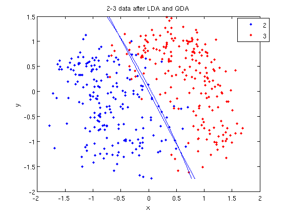
classify can also be used with other discriminant analysis algorithms. The steps laid out above would only need to be modified slightly for those algorithms.

Recall: An analysis of the function of princomp in matlab.
In our assignment 1, we have learnt that how to perform Principal Component Analysis using SVD method. In fact, the matlab offers us a function called princomp which can perform PCA conveniently. From the matlab help file on princomp, you can find the details about this function. But here we will analyze the code of the function of princomp() in matlab to find something different when comparing with SVD method. The following is the code of princomp and explanations to some emphasized steps.

   function [pc, score, latent, tsquare] = princomp(x);
   %   PRINCOMP Principal Component Analysis (centered and scaled data).
   %   [PC, SCORE, LATENT, TSQUARE] = PRINCOMP(X) takes a data matrix X and
   %   returns the principal components in PC, the so-called Z-scores in SC
   %   ORES, the eigenvalues of the covariance matrix of X in LATENT,
   %   and Hotelling's T-squared statistic for each data point in TSQUARE.
   %   Reference: J. Edward Jackson, A User's Guide to Principal Components
   %   John Wiley & Sons, Inc. 1991 pp. 1-25.
   %   B. Jones 3-17-94
   %   Copyright 1993-2002 The MathWorks, Inc.
   %   $Revision: 2.9 $  $Date: 2002/01/17 21:31:45 $
   [m,n] = size(x);       %  get the lengh of the rows and columns of matrix x. 
   r = min(m-1,n);        %  max possible rank of X                    
   avg = mean(x);         %  the mean of every column of X
   centerx = (x - avg(ones(m,1),:));     
                          %  centers X by subtracting off column means                 
   [U,latent,pc] = svd(centerx./sqrt(m-1),0);                          
                          %  "economy size" decomposition
   score = centerx*pc;      
                          %  the representation of X in the principal component space
   if nargout < 3
      return;
    end
    latent = diag(latent).^2;
    if (r   latent = [latent(1:r); zeros(n-r,1)];
    score(:,r+1:end) = 0;
    end
    if nargout < 4
    return;
    end
    tmp = sqrt(diag(1./latent(1:r)))*score(:,1:r)';
    tsquare = sum(tmp.*tmp)';

From the above code, we should pay attention to the following aspects when comparing with SVD method:

First, Rows of [math]\displaystyle{ \,X }[/math] correspond to observations, columns to variables. When using princomp on 2_3 data in assignment 1, note that we take the transpose of [math]\displaystyle{ \,X }[/math].

 >> load 2_3;
 >> [U, score] = princomp(X');

Second, princomp centers X by subtracting off column means.

The third, when [math]\displaystyle{ \,X=UdV' }[/math], princomp uses [math]\displaystyle{ \,V }[/math] as coefficients for principal components, rather than [math]\displaystyle{ \,U }[/math].

The following is an example to perform PCA using princomp and SVD respectively to get the same results.

SVD method

 >> load 2_3
 >> mn=mean(X,2);
 >> X1=X-repmat(mn,1,400);
 >> [s d v]=svd(X1');
 >> y=X1'*v;

princomp

 >>[U score]=princomp(X');

Then we can see that y=score, v=U.

Trick: Using LDA to do QDA - October 7, 2009

There is a trick that allows us to use the linear discriminant analysis (LDA) algorithm to generate as its output a quadratic function that can be used to classify data. This trick is similar to, but more primitive than, the Kernel trick that will be discussed later in the course.

Essentially, the trick involves adding one or more new features (i.e. new dimensions) that just contain our original data projected to that dimension. We then do LDA on our new higher-dimensional data. The answer provided by LDA can then be collapsed onto a lower dimension, giving us a quadratic answer.

Motivation

Why would we want to use LDA over QDA? In situations where we have fewer data points, LDA turns out to be more robust.

If we look back at the equations for LDA and QDA, we see that in LDA we must estimate [math]\displaystyle{ \,\mu_1 }[/math], [math]\displaystyle{ \,\mu_2 }[/math] and [math]\displaystyle{ \,\Sigma }[/math]. In QDA we must estimate all of those, plus another [math]\displaystyle{ \,\Sigma }[/math]; the extra [math]\displaystyle{ \,\frac{d(d-1)}{2} }[/math] estimations make QDA less robust with fewer data points.

Theoretically

Suppose we can estimate some vector [math]\displaystyle{ \underline{w}^T }[/math] such that

[math]\displaystyle{ y = \underline{w}^Tx }[/math]

where [math]\displaystyle{ \underline{w} }[/math] is a d-dimensional column vector, and [math]\displaystyle{ x\ \epsilon\ \Re^d }[/math] (vector in d dimensions).

We also have a non-linear function [math]\displaystyle{ g(x) = y = x^Tvx + \underline{w}^Tx }[/math] that we cannot estimate.

Using our trick, we create two new vectors, [math]\displaystyle{ \,\underline{w}^* }[/math] and [math]\displaystyle{ \,x^* }[/math] such that:

[math]\displaystyle{ \underline{w}^{*T} = [w_1,w_2,...,w_d,v_1,v_2,...,v_d] }[/math]

and

[math]\displaystyle{ x^{*T} = [x_1,x_2,...,x_d,{x_1}^2,{x_2}^2,...,{x_d}^2] }[/math]

We can then estimate a new function, [math]\displaystyle{ g^*(x,x^2) = y^* = \underline{w}^{*T}x^* }[/math].

Note that we can do this for any [math]\displaystyle{ x }[/math] and in any dimension; we could extend a [math]\displaystyle{ D \times n }[/math] matrix to a quadratic dimension by appending another [math]\displaystyle{ D \times n }[/math] matrix with the original matrix squared, to a cubic dimension with the original matrix cubed, or even with a different function altogether, such as a [math]\displaystyle{ \,sin(x) }[/math] dimension.

By Example

Let's use our trick to do a quadratic analysis of the 2_3 data using LDA.

>> load 2_3;
>> [U, sample] = princomp(X');
>> sample = sample(:,1:2);

We start off the same way, by using PCA to reduce the dimensionality of our data to 2.

>> X_star = zeros(400,4);
>> X_star(:,1:2) = sample(:,:);
>> for i=1:400
     for j=1:2
       X_star(i,j+2) = X_star(i,j)^2;
     end
   end

This projects our sample into two more dimensions by squaring our initial two dimensional data set.

>> group = ones(400,1);
>> group(201:400) = 2;
>> [class, error, POSTERIOR, logp, coeff] = classify(X_star, X_star, group, 'linear');
>> sum (class==group)
ans =
   375

We can now display our results.

>> k = coeff(1,2).const;
>> l = coeff(1,2).linear;
>> f = sprintf('0 = %g+%g*x+%g*y+%g*(x)^2+%g*(y)^2', k, l(1), l(2),l(3),l(4));
>> ezplot(f,[min(sample(:,1)), max(sample(:,1)), min(sample(:,2)), max(sample(:,2))]);

The plot shows the quadratic decision boundary obtained using LDA in the four-dimensional space on the 2_3.mat data. Counting the blue and red points that are on the wrong side of the decision boundary, we can confirm that we have correctly classified 375 data points.

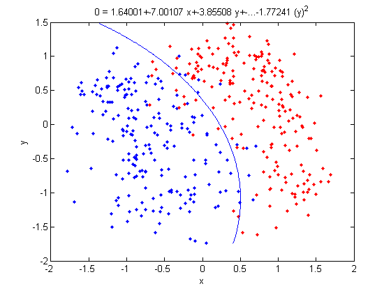
Not only does LDA give us a better result than it did previously, it actually beats QDA, which only correctly classified 371 data points for this data set. Continuing this procedure by adding another two dimensions with [math]\displaystyle{ x^4 }[/math] (i.e. we set X_star(i,j+2) = X_star(i,j)^4) we can correctly classify 376 points.

Introduction to Fisher's Discriminant Analysis - October 7, 2009

Fisher's Discriminant Analysis (FDA), also known as Fisher's Linear Discriminant Analysis (LDA) in some sources, is a classical feature extraction technique. It was originally described in 1936 by Sir Ronald Aylmer Fisher, an English statistician and eugenicist who has been described as one of the founders of modern statistical science. His original paper describing FDA can be found here; a Wikipedia article summarizing the algorithm can be found here.

Contrasting FDA with PCA

The goal of FDA is in contrast to our other main feature extraction technique, principal component analysis (PCA).

• In PCA, we map data to lower dimensions to maximize the variation in those dimensions.
• In FDA, we map data to lower dimensions to best separate data in different classes.

2 clouds of data, and the lines that might be produced by PCA and FDA.

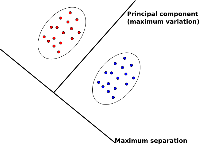
Because we are concerned with identifying which class data belongs to, FDA is often a better feature extraction algorithm for classification.

Another difference between PCA and FDA is that FDA is a supervised algorithm; that is, we know what class data belongs to, and we exploit that knowledge to find a good projection to lower dimensions.

Intuitive Description of FDA

An intuitive description of FDA can be given by visualizing two clouds of data, as shown above. Ideally, we would like to collapse all of the data points in each cloud onto one point on some projected line, then make those two points as far apart as possible. In doing so, we make it very easy to tell which class a data point belongs to. In practice, it is not possible to collapse all of the points in a cloud to one point, but we attempt to make all of the points in a cloud close to each other while simultaneously far from the points in the other cloud.

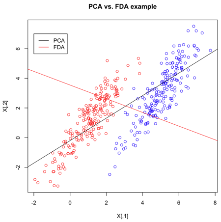
Example in R

PCA and FDA primary dimension for normal multivariate data, using R.

>> X = matrix(nrow=400,ncol=2)
>> X[1:200,] = mvrnorm(n=200,mu=c(1,1),Sigma=matrix(c(1,1.5,1.5,3),2))
>> X[201:400,] = mvrnorm(n=200,mu=c(5,3),Sigma=matrix(c(1,1.5,1.5,3),2))
>> Y = c(rep("red",200),rep("blue",200))

Create 2 multivariate normal random variables with [math]\displaystyle{ \, \mu_1 = \left( \begin{array}{c}1 \\ 1 \end{array} \right), \mu_2 = \left( \begin{array}{c}5 \\ 3 \end{array} \right). ~\textrm{Cov} = \left( \begin{array}{cc} 1 & 1.5 \\ 1.5 & 3 \end{array} \right) }[/math]. Create Y, an index indicating which class they belong to.

>> s <- svd(X,nu=1,nv=1)

Calculate the singular value decomposition of X. The most significant direction is in s$v[,1], and is displayed as a black line.

>> s2 <- lda(X,grouping=Y)

The lda function, given the group for each item, uses Fischer's Linear Discriminant Analysis (FLDA) to find the most discriminant direction. This can be found in s2$scaling.

Now that we've calculated the PCA and FLDA decompositions, we create a plot to demonstrate the differences between the two algorithms. FLDA is clearly better suited to discriminating between two classes whereas PCA is primarily good for reducing the number of dimensions when data is high-dimensional.

>> plot(X,col=Y,main="PCA vs. FDA example")

Plot the set of points, according to colours given in Y.

>> slope = s$v[2]/s$v[1]
>> intercept = mean(X[,2])-slope*mean(X[,1])
>> abline(a=intercept,b=slope)

Plot the main PCA direction, drawn through the mean of the dataset. Only the direction is significant.

>> slope2 = s2$scaling[2]/s2$scaling[1]
>> intercept2 = mean(X[,2])-slope2*mean(X[,1])
>> abline(a=intercept2,b=slope2,col="red")

Plot the FLDA direction, again through the mean.

>> legend(-2,7,legend=c("PCA","FDA"),col=c("black","red"),lty=1)

Labeling the lines directly on the graph makes it easier to interpret.

Ficher's Discriminant Analysis (FDA)

The goal of FDA is to reduce the dimensionality of data in order to have separable data points in a new space. We can consider two kinds of problems:

• 2-class problem
• multi-class problem

Two-class problem - October 9, 2009

In the two-class problem, we have the pre-knowledge that data points belong to two classes. Intuitively speaking points of each class form a cloud around the mean of the class, with each class having possibly different size. To be able to separate the two classes we must determine the class whose mean is closest to a given point while also accounting for the different size of each class, which is represented by the covariance of each class.

Assume [math]\displaystyle{ \underline{\mu_{1}}=\frac{1}{n_{1}}\displaystyle\sum_{i:y_{i}=1}\underline{x_{i}} }[/math] and [math]\displaystyle{ \displaystyle\Sigma_{1} }[/math], represent the mean and covariance of the 1st class, and [math]\displaystyle{ \underline{\mu_{2}}=\frac{1}{n_{2}}\displaystyle\sum_{i:y_{i}=2}\underline{x_{i}} }[/math] and [math]\displaystyle{ \displaystyle\Sigma_{2} }[/math] represent the mean and covariance of the 2nd class. We have to find a transformation which satisfies the following goals:

1.To make the means of these two classes as far apart as possible

In other words, the goal is to maximize the distance after projection between class 1 and class 2. This can be done by maximizing the distance between the means of the classes after projection. When projecting the data points to a one-dimensional space, all points will be projected to a single line; the line we seek is the one with the direction that achieves maximum separation of classes upon projetion. If the original points are [math]\displaystyle{ \underline{x_{i}} \in \mathbb{R}^{d} }[/math]and the projected points are [math]\displaystyle{ \underline{w}^T \underline{x_{i}} }[/math] then the mean of the projected points will be [math]\displaystyle{ \underline{w}^T \underline{\mu_{1}} }[/math] and [math]\displaystyle{ \underline{w}^T \underline{\mu_{2}} }[/math] for class 1 and class 2 respectively. The goal now becomes to maximize the Euclidean distance between projected means, [math]\displaystyle{ (\underline{w}^T\underline{\mu_{1}}-\underline{w}^T\underline{\mu_{2}})^T (\underline{w}^T\underline{\mu_{1}}-\underline{w}^T\underline{\mu_{2}}) }[/math]. The steps of this maximization are given below.

2.We want to collapse all data points of each class to a single point, i.e., minimize the covariance within classes

Notice that the variance of the projected classes 1 and 2 are given by [math]\displaystyle{ \underline{w}^T\Sigma_{1}\underline{w} }[/math] and [math]\displaystyle{ \underline{w}^T\Sigma_{2}\underline{w} }[/math]. The second goal is to minimize the sum of these two covariances.

As is demonstrated below, both of these goals can be accomplished simultaneously.

Original points are [math]\displaystyle{ \underline{x_{i}} \in \mathbb{R}^{d} }[/math]
Projected points are [math]\displaystyle{ \underline{z_{i}} \in \mathbb{R}^{1} }[/math] with [math]\displaystyle{ \underline{z_{i}} = \underline{w}^T \cdot\underline{x_{i}} }[/math]

Between class covariance

In this particular case, we want to project all the data points in one dimensional space.

We want to maximize the Euclidean distance between projected means, which is

[math]\displaystyle{ \begin{align} (\underline{w}^T \underline{\mu_{1}} - \underline{w}^T \underline{\mu_{2}})^T(\underline{w}^T \underline{\mu_{1}} - \underline{w}^T \underline{\mu_{2}}) &= (\underline{\mu_{1}}-\underline{\mu_{2}})^T\underline{w} . \underline{w}^T(\underline{\mu_{1}}-\underline{\mu_{2}})\\ &= \underline{w}^T(\underline{\mu_{1}}-\underline{\mu_{2}})(\underline{\mu_{1}}-\underline{\mu_{2}})^T\underline{w} \end{align} }[/math]

The quantity [math]\displaystyle{ (\underline{\mu_{1}}-\underline{\mu_{2}})(\underline{\mu_{1}}-\underline{\mu_{2}})^T }[/math] is called between class covariance or [math]\displaystyle{ \,S_{B} }[/math].

The goal is to maximize : [math]\displaystyle{ \underline{w}^T S_{B} \underline{w} }[/math]

Within class covariance

Covariance of class 1 is [math]\displaystyle{ \,\Sigma_{1} }[/math] Covariance of class 2 is [math]\displaystyle{ \,\Sigma_{2} }[/math] So covariance of projected points will be [math]\displaystyle{ \,\underline{w}^T \Sigma_{1} \underline{w} }[/math] and [math]\displaystyle{ \underline{w}^T \Sigma_{2} \underline{w} }[/math]

If we sum this two quantities we have

[math]\displaystyle{ \begin{align} \underline{w}^T \Sigma_{1} \underline{w} + \underline{w}^T \Sigma_{2} \underline{w} &= \underline{w}^T(\Sigma_{1} + \Sigma_{2})\underline{w} \end{align} }[/math]

The quantity [math]\displaystyle{ \,(\Sigma_{1} + \Sigma_{2}) }[/math] is called within class covariance or [math]\displaystyle{ \,S_{W} }[/math]

The goal is to minimize [math]\displaystyle{ \underline{w}^T S_{W} \underline{w} }[/math]

Objective Function

Instead of maximizing [math]\displaystyle{ \underline{w}^T S_{B} \underline{w} }[/math] and minimizing [math]\displaystyle{ \underline{w}^T S_{W} \underline{w} }[/math] we can define the following objective function:

[math]\displaystyle{ \underset{\underline{w}}{max}\ \frac{\underline{w}^T S_{B} \underline{w}}{\underline{w}^T S_{W} \underline{w}} }[/math]

This maximization problem is equivalent to [math]\displaystyle{ \underset{\underline{w}}{max}\ \underline{w}^T S_{B} \underline{w} }[/math] subject to constraint [math]\displaystyle{ \underline{w}^T S_{W} \underline{w} = 1 }[/math]. We can use the Lagrange multiplier method to solve it:

[math]\displaystyle{ L(\underline{w},\lambda) = \underline{w}^T S_{B} \underline{w} - \lambda(\underline{w}^T S_{W} \underline{w} - 1) }[/math]

With [math]\displaystyle{ \frac{\part L}{\part \underline{w}} = 0 }[/math] we get:

[math]\displaystyle{ \begin{align} &\Rightarrow\ 2\ S_{B}\ \underline{w}\ - 2\lambda\ S_{W}\ \underline{w}\ = 0\\ &\Rightarrow\ S_{B}\ \underline{w}\ =\ \lambda\ S_{W}\ \underline{w} \\ &\Rightarrow\ S_{W}^{-1}\ S_{B}\ \underline{w}\ =\ \lambda\ \underline{w} \end{align} }[/math]

Note that [math]\displaystyle{ \, S_{W}=\Sigma_1+\Sigma_2 }[/math] is sum of two positive matrices and so it has an inverse.

Here [math]\displaystyle{ \underline{w} }[/math] is the eigenvector of [math]\displaystyle{ S_{w}^{-1}\ S_{B} }[/math] corresponding to the largest eigenvalue.

In facts, this expression can be simplified even more.

[math]\displaystyle{ \Rightarrow\ S_{w}^{-1}\ S_{B}\ \underline{w}\ =\ \lambda\ \underline{w} }[/math] with [math]\displaystyle{ S_{B}\ =\ (\underline{\mu_{1}}-\underline{\mu_{2}})(\underline{\mu_{1}}-\underline{\mu_{2}})^T }[/math]

[math]\displaystyle{ \Rightarrow\ S_{w}^{-1}\ (\underline{\mu_{1}}-\underline{\mu_{2}})(\underline{\mu_{1}}-\underline{\mu_{2}})^T \underline{w}\ =\ \lambda\ \underline{w} }[/math]

The quantity [math]\displaystyle{ (\underline{\mu_{1}}-\underline{\mu_{2}})^T \underline{w} }[/math] and [math]\displaystyle{ \lambda }[/math] are scalars.
So we can say the quantity [math]\displaystyle{ S_{w}^{-1}\ (\underline{\mu_{1}}-\underline{\mu_{2}}) }[/math] is proportional to [math]\displaystyle{ \underline{w} }[/math]

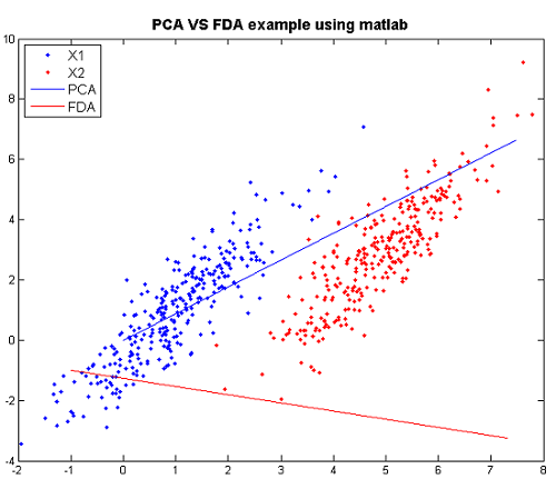
FDA vs. PCA Example in Matlab

We can compare PCA and FDA through the figure produced by matlab.

The following are the code to produce the figure step by step and the explanation for steps.

 >>X1=mvnrnd([1,1],[1 1.5;1.5 3],300);
 >>X2=mvnrnd([5,3],[1 1.5;1.5 3],300);
 >>X=[X1;X2];

Create two multivariate normal random variables with [math]\displaystyle{ \, \mu_1 = \left( \begin{array}{c}1 \\ 1 \end{array} \right), \mu_2 = \left( \begin{array}{c}5 \\ 3 \end{array} \right). ~\textrm{Cov} = \left( \begin{array}{cc} 1 & 1.5 \\ 1.5 & 3 \end{array} \right) }[/math].

 >>plot(X(1:300,1),X(1:300,2),'.');
 >>hold on
 >>p1=plot(X(301:600,1),X(301:600,2),'r.');

Plot the the data of the two classes respectively.

 >>[U Y]=princomp(X);
 >>plot([0 U(1,1)*10],[0 U(2,1)*10]);

Using PCA to find the principal component and plot it.

 >>sw=2*[1 1.5;1.5 3];
 >>sb=([1; 1]-[5 ;3])*([1; 1]-[5; 3])';
 >>g =inv(sw)*sb;
 >>[v w]=eigs(g);
 >>plot([v(1,1)*5 0],[v(2,1)*5 0],'r')

Using FDA to find the principal component and plot it.

Now we can compare them through the figure.

PCA and FDA primary dimension for normal multivariate data, using matlab

Practical example of 2_3

In this matlab example we explore FDA using our familiar data set 2_3 which consists of 200 handwritten "2" and 200 handwritten "3".

X is a matrix of size 64*400 and each column represents an 8*8 image of "2" or "3". Here X1 gets all "2" and X2 gets all "3".

>>load 2_3
>>X1 = X(:, 1:200);
>>X2 = X(:, 201:400);

Next we calculate within class covariance and between class covariance as before.

>>mu1 = mean(X1, 2);
>>mu2 = mean(X2, 2);
>>sb = (mu1 - mu2) * (mu1 - mu2)';
>>sw = cov(X1') + cov(X2');

We use the first two eigenvectors to project the dato in a two-dimensional space.

>>[v d] = eigs( inv(sw) * sb );
>>w = v(:, 1:2);
>>X_hat = w'*X;

Finally we plot the data and visualize the effect of FDA.

>> scatter(ones(1,200),X_hat(1:200))
>> hold on
>> scatter(ones(1,200),X_hat(201:400),'r')

File:fda2-3.jpg

FDA projection of data 2_3, using Matlab.

FDA for Multi-class Problems - October 14, 2009

For the [math]\displaystyle{ k }[/math]-class problem, we need to find a projection from [math]\displaystyle{ d }[/math]-dimensional space to a [math]\displaystyle{ (k-1) }[/math]-dimensional space.

Basically, the within class covariance matrix [math]\displaystyle{ \mathbf{S}_{W} }[/math] is easily to obtain:

[math]\displaystyle{ \begin{align} \mathbf{S}_{W} = \sum_{i=1}^{k} \mathbf{S}_{W,i} \end{align} }[/math]

where [math]\displaystyle{ \mathbf{S}_{W,i} = \frac{1}{n_{i}}\sum_{j: y_{j}=i}(\mathbf{x}_{j} - \mathbf{\mu}_{i})(\mathbf{x}_{j} - \mathbf{\mu}_{i})^{T} }[/math] and [math]\displaystyle{ \mathbf{\mu}_{i} = \frac{\sum_{j: y_{j}=i}\mathbf{x}_{j}}{n_{i}} }[/math].

However, the between class covariance matrix [math]\displaystyle{ \mathbf{S}_{B} }[/math] is not easy to obtain. One of the simplifications is that we may assume that the total covariance [math]\displaystyle{ \mathbf{S}_{T} }[/math] of the data is constant, since [math]\displaystyle{ \mathbf{S}_{W} }[/math] is easy to compute, we can get [math]\displaystyle{ \mathbf{S}_{B} }[/math] using the following relationship:

[math]\displaystyle{ \begin{align} \mathbf{S}_{B} = \mathbf{S}_{T} - \mathbf{S}_{W} \end{align} }[/math]

Actually, there is another generation for [math]\displaystyle{ \mathbf{S}_{B} }[/math]. Denote a total mean vector [math]\displaystyle{ \mathbf{\mu} }[/math] by

[math]\displaystyle{ \begin{align} \mathbf{\mu} = \frac{1}{n}\sum_{i}\mathbf{x_{i}} = \frac{1}{n}\sum_{j=1}^{k}n_{j}\mathbf{\mu}_{j} \end{align} }[/math]

Thus the total covariance matrix [math]\displaystyle{ \mathbf{S}_{T} }[/math] is

[math]\displaystyle{ \begin{align} \mathbf{S}_{T} = \sum_{i}(\mathbf{x_{i}-\mu})(\mathbf{x_{i}-\mu})^{T} \end{align} }[/math]

Thus we obtain

[math]\displaystyle{ \begin{align} & \mathbf{S}_{T} = \sum_{i=1}^{k}\sum_{j: y_{j}=i}(\mathbf{x}_{j} - \mathbf{\mu}_{i} + \mathbf{\mu}_{i} - \mathbf{\mu})(\mathbf{x}_{j} - \mathbf{\mu}_{i} + \mathbf{\mu}_{i} - \mathbf{\mu})^{T} \\& = \sum_{i=1}^{k}\sum_{j: y_{j}=i}(\mathbf{x}_{j}-\mathbf{\mu}_{i})(\mathbf{x}_{j}-\mathbf{\mu}_{i})^{T}+ \sum_{i=1}^{k}\sum_{j: y_{j}=i}(\mathbf{\mu}_{i}-\mathbf{\mu})(\mathbf{\mu}_{i}-\mathbf{\mu})^{T} \\& = \mathbf{S}_{W} + \sum_{i=1}^{k} n_{i}(\mathbf{\mu}_{i}-\mathbf{\mu})(\mathbf{\mu}_{i}-\mathbf{\mu})^{T} \end{align} }[/math]

Since the total covariance [math]\displaystyle{ \mathbf{S}_{T} }[/math] is the sum of the within class covariance [math]\displaystyle{ \mathbf{S}_{W} }[/math] and the between class covariance [math]\displaystyle{ \mathbf{S}_{B} }[/math], we can denote the second term as the general between class covariance matrix [math]\displaystyle{ \mathbf{S}_{B} }[/math], thus we obtain

[math]\displaystyle{ \begin{align} \mathbf{S}_{B} = \sum_{i=1}^{k} n_{i}(\mathbf{\mu}_{i}-\mathbf{\mu})(\mathbf{\mu}_{i}-\mathbf{\mu})^{T} \end{align} }[/math]

Therefore,

[math]\displaystyle{ \begin{align} \mathbf{S}_{T} = \mathbf{S}_{W} + \mathbf{S}_{B} \end{align} }[/math]

Recall that in the two class case problem, we have

[math]\displaystyle{ \begin{align} & \mathbf{S}_{B^{\ast}} = (\mathbf{\mu}_{1}-\mathbf{\mu}_{2})(\mathbf{\mu}_{1}-\mathbf{\mu}_{2})^{T} \\ & = (\mathbf{\mu}_{1}-\mathbf{\mu}+\mathbf{\mu}-\mathbf{\mu}_{2})(\mathbf{\mu}_{1}-\mathbf{\mu}+\mathbf{\mu}-\mathbf{\mu}_{2})^{T} \\ & = ((\mathbf{\mu}_{1}-\mathbf{\mu})-(\mathbf{\mu}_{2}-\mathbf{\mu}))((\mathbf{\mu}_{1}-\mathbf{\mu})-(\mathbf{\mu}_{2}-\mathbf{\mu}))^{T} \\ & = (\mathbf{\mu}_{1}-\mathbf{\mu})(\mathbf{\mu}_{1}-\mathbf{\mu})^{T}+(\mathbf{\mu}_{2}-\mathbf{\mu})(\mathbf{\mu}_{2}-\mathbf{\mu})^{T} \end{align} }[/math]

From the general form,

[math]\displaystyle{ \begin{align} & \mathbf{S}_{B} = n_{1}(\mathbf{\mu}_{1}-\mathbf{\mu})(\mathbf{\mu}_{1}-\mathbf{\mu})^{T} + n_{2}(\mathbf{\mu}_{2}-\mathbf{\mu})(\mathbf{\mu}_{2}-\mathbf{\mu})^{T} \end{align} }[/math]

Apparently, they are very similar.

Now, we are trying to find the optimal transformation. Basically, we have

[math]\displaystyle{ \begin{align} \mathbf{z}_{i} = \mathbf{W}^{T}\mathbf{x}_{i}, i=1,2,...,k-1 \end{align} }[/math]

where [math]\displaystyle{ \mathbf{z}_{i} }[/math] is a [math]\displaystyle{ (k-1)\times 1 }[/math] vector, [math]\displaystyle{ \mathbf{W} }[/math] is a [math]\displaystyle{ d\times (k-1) }[/math] transformation matrix, i.e. [math]\displaystyle{ \mathbf{W} = [\mathbf{w}_{1}, \mathbf{w}_{2},..., \mathbf{w}_{k-1}] }[/math], and [math]\displaystyle{ \mathbf{x}_{i} }[/math] is a [math]\displaystyle{ d\times 1 }[/math] column vector.

Thus we obtain

[math]\displaystyle{ \begin{align} & \mathbf{S}_{W}^{\ast} = \sum_{i=1}^{k}\sum_{j: y_{j}=i}(\mathbf{W}^{T}\mathbf{x}_{j}-\mathbf{W}^{T}\mathbf{\mu}_{i})(\mathbf{W}^{T}\mathbf{x}_{j}-\mathbf{W}^{T}\mathbf{\mu}_{i})^{T} \\ & = \sum_{i=1}^{k}\sum_{j: y_{j}=i}\mathbf{W}^{T}(\mathbf{x}_{j}-\mathbf{\mu}_{i})(\mathbf{x}_{j}-\mathbf{\mu}_{i})\mathbf{W} \\ & = \mathbf{W}^{T}\left[\sum_{i=1}^{k}\sum_{j: y_{j}=i}(\mathbf{x}_{j}-\mathbf{\mu}_{i})(\mathbf{x}_{j}-\mathbf{\mu}_{i})\right]\mathbf{W} \\ & = \mathbf{W}^{T}\mathbf{S}_{W}\mathbf{W} \end{align} }[/math]

Similarly, we obtain

[math]\displaystyle{ \begin{align} & \mathbf{S}_{B}^{\ast} = \sum_{i=1}^{k}n_{i}(\mathbf{W}^{T}\mathbf{\mu}_{i}-\mathbf{W}^{T}\mathbf{\mu})(\mathbf{W}^{T}\mathbf{\mu}_{i}-\mathbf{W}^{T}\mathbf{\mu})^{T} \\ & = \sum_{i=1}^{k}n_{i}\mathbf{W}^{T}(\mathbf{\mu}_{i}-\mathbf{\mu})(\mathbf{\mu}_{i}-\mathbf{\mu})^{T}\mathbf{W} \\ & = \mathbf{W}^{T}\left[ \sum_{i=1}^{k}n_{i}(\mathbf{\mu}_{i}-\mathbf{\mu})(\mathbf{\mu}_{i}-\mathbf{\mu})^{T}\right]\mathbf{W} \\ & = \mathbf{W}^{T}\mathbf{S}_{B}\mathbf{W} \end{align} }[/math]

Now, we use the determinant of the matrix, i.e. the product of the eigenvalues of the matrix, as our measure.

[math]\displaystyle{ \begin{align} \phi(\mathbf{W}) = \frac{|\mathbf{S}_{B}^{\ast}|}{|\mathbf{S}_{W}^{\ast}|} = \frac{\mathbf{W}^{T}\mathbf{S}_{B}\mathbf{W}}{\mathbf{W}^{T}\mathbf{S}_{W}\mathbf{W}} \end{align} }[/math]

The solution for this question is that the columns of the transformation matrix [math]\displaystyle{ \mathbf{W} }[/math] are exactly the eigenvectors that correspond to largest [math]\displaystyle{ k-1 }[/math] eigenvalues with respect to

[math]\displaystyle{ \begin{align} \mathbf{S}_{W}^{-1}\mathbf{S}_{B}\mathbf{w}_{i} = \lambda_{i}\mathbf{w}_{i} \end{align} }[/math]

Also, note that we can use

[math]\displaystyle{ \begin{align} \sum_{i=1}^{k}n_{i}\|(\mathbf{W}^{T}\mathbf{\mu}_{i}-\mathbf{W}^{T}\mathbf{\mu})^{T}\|^{2} \end{align} }[/math]

as our measure.

Recall that

[math]\displaystyle{ \begin{align} \|\mathbf{X}\|^2 = Tr(\mathbf{X}^{T}\mathbf{X}) \end{align} }[/math]

Thus we obtain that

[math]\displaystyle{ \begin{align} & \sum_{i=1}^{k}n_{i}\|(\mathbf{W}^{T}\mathbf{\mu}_{i}-\mathbf{W}^{T}\mathbf{\mu})^{T}\|^{2} \\ & = \sum_{i=1}^{k}n_{i}Tr[(\mathbf{W}^{T}\mathbf{\mu}_{i}-\mathbf{W}^{T}\mathbf{\mu})(\mathbf{W}^{T}\mathbf{\mu}_{i}-\mathbf{W}^{T}\mathbf{\mu})^{T}] \\ & = Tr[\sum_{i=1}^{k}n_{i}(\mathbf{W}^{T}\mathbf{\mu}_{i}-\mathbf{W}^{T}\mathbf{\mu})(\mathbf{W}^{T}\mathbf{\mu}_{i}-\mathbf{W}^{T}\mathbf{\mu})^{T}] \\ & = Tr[\sum_{i=1}^{k}n_{i}\mathbf{W}^{T}(\mathbf{\mu}_{i}-\mathbf{\mu})(\mathbf{\mu}_{i}-\mathbf{\mu})^{T}\mathbf{W}] \\ & = Tr[\mathbf{W}^{T}\sum_{i=1}^{k}n_{i}(\mathbf{\mu}_{i}-\mathbf{\mu})(\mathbf{\mu}_{i}-\mathbf{\mu})^{T}\mathbf{W}] \\ & = Tr[\mathbf{W}^{T}\mathbf{S}_{B}\mathbf{W}] \end{align} }[/math]

Similarly, we can get [math]\displaystyle{ Tr[\mathbf{W}^{T}\mathbf{S}_{W}\mathbf{W}] }[/math]. Thus we have following criterion function

[math]\displaystyle{ \begin{align} \phi(\mathbf{W}) = \frac{Tr[\mathbf{W}^{T}\mathbf{S}_{B}\mathbf{W}]}{Tr[\mathbf{W}^{T}\mathbf{S}_{W}\mathbf{W}]} \end{align} }[/math]

Similar to the two class case problem, we have:

max [math]\displaystyle{ Tr[\mathbf{W}^{T}\mathbf{S}_{B}\mathbf{W}] }[/math] subject to [math]\displaystyle{ Tr[\mathbf{W}^{T}\mathbf{S}_{W}\mathbf{W}]=1 }[/math]

To solve this optimization problem a Lagrange multiplier [math]\displaystyle{ \Lambda }[/math], which actually is a [math]\displaystyle{ d \times d }[/math] diagonal matrix, is introduced:

[math]\displaystyle{ \begin{align} L(\mathbf{W},\Lambda) = Tr[\mathbf{W}^{T}\mathbf{S}_{W}\mathbf{B}] - \Lambda\left\{ Tr[\mathbf{W}^{T}\mathbf{S}_{W}\mathbf{W}] - 1 \right\} \end{align} }[/math]

Differentiating with respect to [math]\displaystyle{ \mathbf{W} }[/math] we obtain:

[math]\displaystyle{ \begin{align} \frac{\partial L}{\partial \mathbf{W}} = (\mathbf{S}_{B} + \mathbf{S}_{B}^{T})\mathbf{W} - \Lambda (\mathbf{S}_{W} + \mathbf{S}_{W}^{T})\mathbf{W} \end{align} }[/math]

Note that the [math]\displaystyle{ \mathbf{S}_{B} }[/math] and [math]\displaystyle{ \mathbf{S}_{W} }[/math] are both symmetric matrices, thus set the first derivative to zero, we obtain:

[math]\displaystyle{ \begin{align} \mathbf{S}_{B}\mathbf{W} - \Lambda\mathbf{S}_{W}\mathbf{W}=0 \end{align} }[/math]

Thus,

[math]\displaystyle{ \begin{align} \mathbf{S}_{B}\mathbf{W} = \Lambda\mathbf{S}_{W}\mathbf{W} \end{align} }[/math]

where

[math]\displaystyle{ \mathbf{\Lambda} = \begin{pmatrix} \lambda_{1} & & 0\\ &\ddots&\\ 0 & &\lambda_{d} \end{pmatrix} }[/math]

and [math]\displaystyle{ \mathbf{W} = [\mathbf{w}_{1}, \mathbf{w}_{2},..., \mathbf{w}_{k-1}] }[/math].

As a matter of fact, [math]\displaystyle{ \mathbf{\Lambda} }[/math] must have [math]\displaystyle{ \mathbf{k-1} }[/math] nonzero eigenvalues, because [math]\displaystyle{ rank({S}_{W}^{-1}\mathbf{S}_{B})=k-1 }[/math].

Therefore, the solution for this question is as same as the previous case. The columns of the transformation matrix [math]\displaystyle{ \mathbf{W} }[/math] are exactly the eigenvectors that correspond to largest [math]\displaystyle{ k-1 }[/math] eigenvalues with respect to

[math]\displaystyle{ \begin{align} \mathbf{S}_{W}^{-1}\mathbf{S}_{B}\mathbf{w}_{i} = \lambda_{i}\mathbf{w}_{i} \end{align} }[/math]

Linear Regression Models - October 14, 2009

Regression analysis is a general statistical technique for modelling and analyzing how a dependent variable changes according to changes in independent variables. In classification, we are interested in how a label, [math]\displaystyle{ \,y }[/math], changes according to changes in [math]\displaystyle{ \,X }[/math].

We will start by considering a very simple regression model, the linear regression model.

General information on linear regression can be found at the University of South Florida and this MIT lecture.

For the purpose of classification, the linear regression model assumes that the regression function [math]\displaystyle{ \,E(Y|X) }[/math] is linear in the inputs [math]\displaystyle{ \,\mathbf{x}_{1}, ..., \mathbf{x}_{p} }[/math].

The linear regression model has the general form:

[math]\displaystyle{ \begin{align} f(x) = \beta^{T}\mathbf{x}_{i}+\beta_{0} \end{align} }[/math]

where [math]\displaystyle{ \,\beta }[/math] is a [math]\displaystyle{ 1 \times d }[/math] vector.

Given input data [math]\displaystyle{ \,\mathbf{x}_{1}, ..., \mathbf{x}_{p} }[/math] and [math]\displaystyle{ \,y_{1}, ..., y_{p} }[/math] our goal is to find [math]\displaystyle{ \,\beta }[/math] and [math]\displaystyle{ \,\beta_0 }[/math] such that the linear model fits the data while minimizing sum of squared errors using the Least Squares method.

Note that vectors [math]\displaystyle{ \mathbf{x}_{i} }[/math] could be numerical inputs, transformations of the original data, i.e. [math]\displaystyle{ \log \mathbf{x}_{i} }[/math] or [math]\displaystyle{ \sin \mathbf{x}_{i} }[/math], or basis expansions, i.e. [math]\displaystyle{ \mathbf{x}_{i}^{2} }[/math] or [math]\displaystyle{ \mathbf{x}_{i}\times \mathbf{x}_{j} }[/math].

Denote [math]\displaystyle{ \mathbf{X} }[/math] as a [math]\displaystyle{ n\times(d+1) }[/math] matrix with each row an input vector (with 1 in the first position), [math]\displaystyle{ \,\beta = (\beta_0, \beta_1,..., \beta_{d})^{T} }[/math] and [math]\displaystyle{ \mathbf{y} }[/math] as a [math]\displaystyle{ n \times 1 }[/math] vector of outputs. We then try to minimize the residual sum-of-squares

[math]\displaystyle{ \begin{align} \mathrm{RSS}(\beta)=(\mathbf{y}-\mathbf{X}\beta)(\mathbf{y}-\mathbf{X}\beta)^{T} \end{align} }[/math]

This is a quadratic function in the [math]\displaystyle{ \,d+1 }[/math] parameters. Differentiating with respect to [math]\displaystyle{ \,\beta }[/math] we obtain

[math]\displaystyle{ \begin{align} \frac{\partial \mathrm{RSS}}{\partial \beta} = -2\mathbf{X}^{T}(\mathbf{y}-\mathbf{X}\beta) \end{align} }[/math]

[math]\displaystyle{ \begin{align} \frac{\partial^{2}\mathrm{RSS}}{\partial \beta \partial \beta^{T}}=2\mathbf{X}^{T}\mathbf{X} \end{align} }[/math]

Set the first derivative to zero

[math]\displaystyle{ \begin{align} \mathbf{X}^{T}(\mathbf{y}-\mathbf{X}\beta)=0 \end{align} }[/math]

we obtain the solution

[math]\displaystyle{ \begin{align} \hat \beta = (\mathbf{X}^{T}\mathbf{X})^{-1}\mathbf{X}^{T}\mathbf{y} \end{align} }[/math]

Thus the fitted values at the inputs are

[math]\displaystyle{ \begin{align} \mathbf{\hat y} = \mathbf{X}\hat\beta = \mathbf{X} (\mathbf{X}^{T}\mathbf{X})^{-1}\mathbf{X}^{T}\mathbf{y} \end{align} }[/math]

where [math]\displaystyle{ \mathbf{H} = \mathbf{X} (\mathbf{X}^{T}\mathbf{X})^{-1}\mathbf{X}^{T} }[/math] is called the hat matrix.

• Note For classification purposes, this is not a correct model. Recall the following application of Bayes classifier:
  

[math]\displaystyle{ r(x)= P( Y=k | X=x )= \frac{f_{k}(x)\pi_{k}}{\Sigma_{k}f_{k}(x)\pi_{k}} }[/math]
It is clear that to make sense mathematically, [math]\displaystyle{ \displaystyle r(x) }[/math] must be a value between 0 and 1. If this is estimated with the regression function [math]\displaystyle{ \displaystyle r(x)=E(Y|X=x) }[/math] and [math]\displaystyle{ \mathbf{\hat\beta} }[/math] is learned as above, then there is nothing that would restrict [math]\displaystyle{ \displaystyle r(x) }[/math] to taking values between 0 and 1.

A linear regression example in Matlab

We can see how linear regression works through the following example in Matlab. The following is the code and the explanation for each step.

Again, we use the data in 2_3.m.

 >>load 2_3;
 >>[U, sample] = princomp(X');
 >>sample = sample(:,1:2);

We carry out Principal Component Analysis (PCA) to reduce the dimensionality from 64 to 2.

 >>y = zeros(400,1);
 >>y(201:400) = 1;

We let y represent the set of labels coded as 0 and 1.

 >>x=[sample;ones(1,400)];

Construct x by adding a row of vector 1 to data.

 >>b=inv(x*x')*x*y;

Calculate b, which represents [math]\displaystyle{ \beta }[/math] in the linear regression model.

 >>x1=x';
 >>for i=1:400
   if x1(i,:)*b>0.5
        plot(x1(i,1),x1(i,2),'.')
        hold on
   elseif x1(i,:)*b < 0.5
       plot(x1(i,1),x1(i,2),'r.')
   end 
 end

Plot the fitted y values.

File:linearregression.png

the figure shows that the classification of the data points in 2_3.m by the linear regression model

Logistic Regression- October 16, 2009

Intuition behind Logistic Regression

Recall that, for classification purposes, the linear regression model presented in the above section is not correct because it does not force [math]\displaystyle{ \,r(x) }[/math] to be between 0 and 1 and sum to 1. Consider the following log odds model (for two classes):

[math]\displaystyle{ \log\left(\frac{P(Y=1|X=x)}{P(Y=0|X=x)}\right)=\beta^Tx }[/math]

Calculating [math]\displaystyle{ \,P(Y=1|X=x) }[/math] leads us to the logistic regression model, which as opposed to the linear regression model, allows the modeling of the posterior probabilities of the classes through linear methods and at the same time ensures that they sum to one and are between 0 and 1.

This logistic regression model for the two class case is defined as:

[math]\displaystyle{ P(Y=1 | X=x) =\frac{\exp(\underline{\beta}^T \underline{x})}{1+\exp(\underline{\beta}^T \underline{x})} }[/math]

Then we have that [math]\displaystyle{ P(Y=0 | X=x) = 1-P(Y=1 | X=x)=1-\frac{\exp(\underline{\beta}^T \underline{x})}{1+\exp(\underline{\beta}^T \underline{x})}=\frac{1}{1+\exp(\underline{\beta}^T \underline{x})} }[/math]

Logistic regression tries to fit a distribution. The fitting of logistic regression models is usually accomplished by maximum likelihood. The maximum likelihood of [math]\displaystyle{ \underline\beta }[/math] maximizes the probability of obtaining the data [math]\displaystyle{ \displaystyle{x_{1},...,x_{n}} }[/math] from the known distribution. Combining [math]\displaystyle{ \displaystyle P(Y=1 | X=x) }[/math] and [math]\displaystyle{ \displaystyle P(Y=0 | X=x) }[/math] as follows, we can consider the two classes at the same time:

[math]\displaystyle{ \left(\frac{\exp(\underline{\beta}^T \underline{x_i})}{1+\exp(\underline{\beta}^T \underline{x_i})}\right)^y \left(\frac{1}{1+\exp(\underline{\beta}^T \underline{x_i})}\right)^{1-y} }[/math]

Assuming the data [math]\displaystyle{ \displaystyle {x_{1},...,x_{n}} }[/math] is drawn independently, the likelihood function is

[math]\displaystyle{ \begin{align} \mathcal{L}(\theta)&=p({x_{1},...,x_{n}};\theta)\\ &=\displaystyle p(x_{1};\theta) p(x_{2};\theta)... p(x_{n};\theta) \quad \mbox{(by independence)}\\ &= \prod_{i=1}^n p(x_{i};\theta) \end{align} }[/math]

Since it is more convenient to work with the log-likelihood function, take the log of both sides, we get

[math]\displaystyle{ \displaystyle l(\theta)=\displaystyle \sum_{i=1}^n \log p(x_{i};\theta) }[/math]

So,

[math]\displaystyle{ \begin{align} l(\underline\beta)&=\displaystyle\sum_{i=1}^n y_{i}\log\left(\frac{\exp(\underline{\beta}^T \underline{x_i})}{1+\exp(\underline{\beta}^T \underline{x_i})}\right)+(1-y_{i})\log\left(\frac{1}{1+\exp(\underline{\beta}^T\underline{x_i})}\right)\\ &= \displaystyle\sum_{i=1}^n y_{i}(\underline{\beta}^T\underline{x_i}-\log(1+\exp(\underline{\beta}^T\underline{x_i}))+(1-y_{i})(-\log(1+\exp(\underline{\beta}^T\underline{x_i}))\\ &= \displaystyle\sum_{i=1}^n y_{i}\underline{\beta}^T-y_{i} \log(1+\exp(\underline{\beta}^T\underline{x_i}))- \log(1+\exp(\underline{\beta}^T\underline{x_i}))+y_{i} \log(1+\exp(\underline{\beta}^T\underline{x_i}))\\ &=\displaystyle\sum_{i=1}^n y_{i}\underline{\beta}^T- \log(1+\exp(\underline{\beta}^T\underline{x_i}))\\ \end{align} }[/math]

To maximize the log-likelihood, set its derivative to 0.

[math]\displaystyle{ \begin{align} \frac{\partial l}{\partial \underline{\beta}} &= \sum_{i=1}^n \left[{y_i} \underline{x}_i- \frac{\exp(\underline{\beta}^T \underline{x_i})}{1+\exp(\underline{\beta}^T \underline{x}_i)}\underline{x}_i\right]\\ &=\sum_{i=1}^n \left[{y_i} \underline{x}_i - p(\underline{x}_i;\underline{\beta})\underline{x}_i\right] \end{align} }[/math]

To solve this equation, the Newton-Raphson algorithm is used which requires the second derivative in addition to the first derivative. This is demonstrated in the next section.

Logistic Regression(2) - October 19, 2009

Logistic Regression Model

Recall that in the last lecture, we learned the logistic regression model.

• [math]\displaystyle{ P(Y=1 | X=x)=P(\underline{x}_i;\underline{\beta})=\frac{exp(\underline{\beta}^T \underline{x})}{1+exp(\underline{\beta}^T \underline{x})} }[/math]
• [math]\displaystyle{ P(Y=0 | X=x)=1-P(\underline{x}_i;\underline{\beta})=\frac{1}{1+exp(\underline{\beta}^T \underline{x})} }[/math]

Find [math]\displaystyle{ \underline{\beta} }[/math]

Criteria: find a [math]\displaystyle{ \underline{\beta} }[/math] that maximizes the conditional likelihood of Y given X using the training data.

From above, we have the first derivative of the log-likelihood:

[math]\displaystyle{ \frac{\partial l}{\partial \underline{\beta}} = \sum_{i=1}^n \left[{y_i} \underline{x}_i- \frac{exp(\underline{\beta}^T \underline{x_i})}{1+exp(\underline{\beta}^T \underline{x}_i)}\underline{x}_i\right] }[/math] [math]\displaystyle{ =\sum_{i=1}^n \left[{y_i} \underline{x}_i - P(\underline{x}_i;\underline{\beta})\underline{x}_i\right] }[/math]

The Newton-Raphson algorithm requires the second-derivative or Hessian matrix.

[math]\displaystyle{ \frac{\partial^{2} l}{\partial \underline{\beta} \partial \underline{\beta}^T }= \sum_{i=1}^n - \underline{x_i} \frac{(exp(\underline{\beta}^T\underline{x}_i) \underline{x}_i^T)(1+exp(\underline{\beta}^T \underline{x}_i))-\underline{x}_i exp(\underline{\beta}^T\underline{x}_i)exp(\underline{\beta}^T\underline{x}_i)}{(1+exp(\underline{\beta}^T \underline{x}))^2} }[/math]

(note: [math]\displaystyle{ \frac{\partial\underline{\beta}^T\underline{x}_i}{\partial \underline{\beta}^T}=\underline{x}_i^T }[/math] you can check it here, it's a very useful website including a Matrix Reference Manual that you can find information about linear algebra and the properties of real and complex matrices.)

[math]\displaystyle{ =\sum_{i=1}^n - \underline{x}_i \frac{(-\underline{x}_i exp(\underline{\beta}^T\underline{x}_i) \underline{x}_i^T)}{(1+exp(\underline{\beta}^T \underline{x}))(1+exp(\underline{\beta}^T \underline{x}))} }[/math] (by cancellation)

[math]\displaystyle{ =\sum_{i=1}^n - \underline{x}_i \underline{x}_i^T P(\underline{x}_i;\underline{\beta}）)[1-P(\underline{x}_i;\underline{\beta})]） }[/math](since [math]\displaystyle{ P(\underline{x}_i;\underline{\beta})=\frac{exp(\underline{\beta}^T \underline{x})}{1+exp(\underline{\beta}^T \underline{x})} }[/math] and [math]\displaystyle{ 1-P(\underline{x}_i;\underline{\beta})=\frac{1}{1+exp(\underline{\beta}^T \underline{x})} }[/math])

Starting with [math]\displaystyle{ \,\underline{\beta}^{old} }[/math], the Newton-Raphson update is

[math]\displaystyle{ \,\underline{\beta}^{new}\leftarrow \,\underline{\beta}^{old}- (\frac{\partial ^2 l}{\partial \underline{\beta}\partial \underline{\beta}^T})^{-1}(\frac{\partial l}{\partial \underline{\beta}}) }[/math] where the derivatives are evaluated at [math]\displaystyle{ \,\underline{\beta}^{old} }[/math]

The iteration will terminate when [math]\displaystyle{ \underline{\beta}^{new} }[/math] is very close to [math]\displaystyle{ \underline{\beta}^{old} }[/math].

The iteration can be described in matrix form.

• Let [math]\displaystyle{ \,\underline{Y} }[/math] be the column vector of [math]\displaystyle{ \,y_i }[/math]. ([math]\displaystyle{ n\times1 }[/math])
• Let [math]\displaystyle{ \,X }[/math] be the [math]\displaystyle{ {d}\times{n} }[/math] input matrix.
• Let [math]\displaystyle{ \,\underline{P} }[/math] be the [math]\displaystyle{ {n}\times{1} }[/math] vector with [math]\displaystyle{ i }[/math]th element [math]\displaystyle{ P(\underline{x}_i;\underline{\beta}^{old}) }[/math].
• Let [math]\displaystyle{ \,W }[/math] be an [math]\displaystyle{ {n}\times{n} }[/math] diagonal matrix with [math]\displaystyle{ i }[/math]th element [math]\displaystyle{ P(\underline{x}_i;\underline{\beta}^{old})[1-P(\underline{x}_i;\underline{\beta}^{old})] }[/math]

then

[math]\displaystyle{ \frac{\partial l}{\partial \underline{\beta}} = X(\underline{Y}-\underline{P}) }[/math]

[math]\displaystyle{ \frac{\partial ^2 l}{\partial \underline{\beta}\partial \underline{\beta}^T} = -XWX^T }[/math]

The Newton-Raphson step is

[math]\displaystyle{ \underline{\beta}^{new} \leftarrow \underline{\beta}^{old}+(XWX^T)^{-1}X(\underline{Y}-\underline{P}) }[/math]

This equation is sufficient for computation of the logistic regression model. However, we can simplify further to uncover an interesting feature of this equation.

[math]\displaystyle{ \begin{align} \underline{\beta}^{new} &= (XWX^T)^{-1}(XWX^T)\underline{\beta}^{old}+(XWX^T)^{-1}XWW^{-1}(\underline{Y}-\underline{P})\\ &=(XWX^T)^{-1}XW[X^T\underline{\beta}^{old}+W^{-1}(\underline{Y}-\underline{P})]\\ &=(XWX^T)^{-1}XWZ \end{align} }[/math]

where [math]\displaystyle{ Z=X^T\underline{\beta}^{old}+W^{-1}(\underline{Y}-\underline{P}) }[/math]

Recall that linear regression by least square finds the following minimum: [math]\displaystyle{ \min_{\underline{\beta}}(\underline{y}-\underline{\beta}X)^T(\underline{y}-\underline{\beta}^TX) }[/math]

we have [math]\displaystyle{ \underline{\beta}=(XX^T)^{-1}X\underline{y} }[/math]

Similarly, we can say that [math]\displaystyle{ \underline{\beta}^{new} }[/math] is the solution of a weighted least square problem:

[math]\displaystyle{ \underline{\beta}^{new} \leftarrow \min_{\underline{\beta}}(Z-X\underline{\beta}^T)W(Z-X\underline{\beta}) }[/math]

WLS

Actually, the weighted least squares estimator minimizes the weighted error sum of squares [math]\displaystyle{ S(\beta) = \sum_{i=1}^{n}w_{i}[y_{i}-\mathbf{x}_{i}^{T}\beta]^{2} }[/math] where [math]\displaystyle{ w_{i}\gt 0 }[/math]. Hence the WLS estimator is given by [math]\displaystyle{ \hat\beta^{WLS}=\left[\sum_{i=1}^{n}w_{i}\mathbf{x}_{i}\mathbf{x}_{i}^{T} \right]^{-1}\left[ \sum_{i=1}^{n}w_{i}\mathbf{x}_{i}y_{i}\right] }[/math]

note:Here we obtain [math]\displaystyle{ \underline{\beta} }[/math], which is a [math]\displaystyle{ d\times{1} }[/math] vector, because we construct the model like [math]\displaystyle{ \underline{\beta}^T\underline{x} }[/math]. If we construct the model like [math]\displaystyle{ \underline{\beta}_0+ \underline{\beta}^T\underline{x} }[/math], then similar to linear regression, [math]\displaystyle{ \underline{\beta} }[/math] will be a [math]\displaystyle{ (d+1)\times{1} }[/math] vector.

Choosing [math]\displaystyle{ \displaystyle\beta=0 }[/math] seems to be a suitable starting value for the Newton-Raphson iteration procedure in this case. However, this does not guarantee convergence. The procedure will usually converge since the log-likelihood function is concave(or convex). In the case that it does not, we can just prove the local convergence of the method, which means the iteration would converge only if the initial point is closed enough to the exact solution. However, in practice, choosing an appropriate initial value is really trivial, namely, it is not often to find a initial too far from the exact solution to make the iteration invalid. <ref>C. T. Kelley, Iterative Methods for Linear and Nonlinear Equations </ref> Besides, step-size halving will solve this problem. <ref>H. Trevor, R. Tibshirani, J. Friedman, The Elements of Statistical Learning (Springer

2009),121.</ref>

Pseudo Code

1. [math]\displaystyle{ \underline{\beta} \leftarrow 0 }[/math]
2. Set [math]\displaystyle{ \,\underline{Y} }[/math], the label associated with each observation [math]\displaystyle{ \,i=1...n }[/math].
3. Compute [math]\displaystyle{ \,\underline{P} }[/math] according to the equation [math]\displaystyle{ P(\underline{x}_i;\underline{\beta})=\frac{exp(\underline{\beta}^T \underline{x})}{1+exp(\underline{\beta}^T \underline{x})} }[/math] for all [math]\displaystyle{ \,i=1...n }[/math].
4. Compute the diagonal matrix [math]\displaystyle{ \,W }[/math] by setting [math]\displaystyle{ \,w_i,i }[/math] to [math]\displaystyle{ P(\underline{x}_i;\underline{\beta}）)[1-P(\underline{x}_i;\underline{\beta})] }[/math] for all [math]\displaystyle{ \,i=1...n }[/math].
5. [math]\displaystyle{ Z \leftarrow X^T\underline{\beta}+W^{-1}(\underline{Y}-\underline{P}) }[/math].
6. [math]\displaystyle{ \underline{\beta} \leftarrow (XWX^T)^{-1}XWZ }[/math].
7. If the new [math]\displaystyle{ \underline{\beta} }[/math] value is sufficiently close to the old value, stop; otherwise go back to step 3.

Comparison with Linear Regression

• Similarities

1. They are both to attempt to estimate [math]\displaystyle{ \,P(Y=k|X=x) }[/math] (For logistic regression, we just mentioned about the case that [math]\displaystyle{ \,k=0 }[/math] or [math]\displaystyle{ \,k=1 }[/math] now).
2. They are both have linear boundaris.

note:For linear regression, we assume the model is linear. The boundary is [math]\displaystyle{ P(Y=k|X=x)=\underline{\beta}^T\underline{x}_i+\underline{\beta}_0=0.5 }[/math] (linear)

For logistic regression, the boundary is [math]\displaystyle{ P(Y=k|X=x)=\frac{exp(\underline{\beta}^T \underline{x})}{1+exp(\underline{\beta}^T \underline{x})}=0.5 \Rightarrow exp(\underline{\beta}^T \underline{x})=1\Rightarrow \underline{\beta}^T \underline{x}=0 }[/math] (linear)

• Differences

1. Linear regression: [math]\displaystyle{ \,P(Y=k|X=x) }[/math] is linear function of [math]\displaystyle{ \,x }[/math], [math]\displaystyle{ \,P(Y=k|X=x) }[/math] is not guaranteed to fall between 0 and 1 and to sum up to 1.
2. Logistic regression: [math]\displaystyle{ \,P(Y=k|X=x) }[/math] is a nonlinear function of [math]\displaystyle{ \,x }[/math], and it is guaranteed to range from 0 to 1 and to sum up to 1.

Comparison with LDA

1. The linear logistic model only consider the conditional distribution [math]\displaystyle{ \,P(Y=k|X=x) }[/math]. No assumption is made about [math]\displaystyle{ \,P(X=x) }[/math].
2. The LDA model specifies the joint distribution of [math]\displaystyle{ \,X }[/math] and [math]\displaystyle{ \,Y }[/math].
3. Logistic regression maximizes the conditional likelihood of [math]\displaystyle{ \,Y }[/math] given [math]\displaystyle{ \,X }[/math]: [math]\displaystyle{ \,P(Y=k|X=x) }[/math]
4. LDA maximizes the joint likelihood of [math]\displaystyle{ \,Y }[/math] and [math]\displaystyle{ \,X }[/math]: [math]\displaystyle{ \,P(Y=k,X=x) }[/math].
5. If [math]\displaystyle{ \,\underline{x} }[/math] is d-dimensional,the number of adjustable parameter in logistic regression is [math]\displaystyle{ \,d }[/math]. The number of parameters grows linearly w.r.t dimension.
6. If [math]\displaystyle{ \,\underline{x} }[/math] is d-dimensional,the number of adjustable parameter in LDA is [math]\displaystyle{ \,(2d)+d(d+1)/2+2=(d^2+5d+4)/2 }[/math]. The number of parameters grows quardratically w.r.t dimension.
7. As logistic regression relies on fewer assumptions, it seems to be more robust.
8. In practice, Logistic regression and LDA often give the similar results.

By example

Now we compare LDA and Logistic regression by an example. Again, we use them on the 2_3 data.

 >>load 2_3;
 >>[U, sample] = princomp(X');
 >>sample = sample(:,1:2);
 >>plot (sample(1:200,1), sample(1:200,2), '.');
 >>hold on;
 >>plot (sample(201:400,1), sample(201:400,2), 'r.'); 

First, we do PCA on the data and plot the data points that represent 2 or 3 in different colors. See the previous example for more details.

 >>group = ones(400,1);
 >>group(201:400) = 2;

Group the data points.

 >>[B,dev,stats] = mnrfit(sample,group);
 >>x=[ones(1,400); sample'];

Now we use mnrfit to use logistic regression to classfy the data. This function can return B which is a [math]\displaystyle{ (d+1)\times{(k–1)} }[/math] matrix of estimates, where each column corresponds to the estimated intercept term and predictor coefficients. In this case, B is a [math]\displaystyle{ 3\times{1} }[/math] matrix.

 >> B
 B =0.1861
   -5.5917
   -3.0547

This is our [math]\displaystyle{ \underline{\beta} }[/math]. So the posterior probabilities are:

[math]\displaystyle{ P(Y=1 | X=x)=\frac{exp(0.1861-5.5917X_1-3.0547X_2)}{1+exp(0.1861-5.5917X_1-3.0547X_2)} }[/math].

[math]\displaystyle{ P(Y=2 | X=x)=\frac{1}{1+exp(0.1861-5.5917X_1-3.0547X_2)} }[/math]

The classification rule is:

[math]\displaystyle{ \hat Y = 1 }[/math], if [math]\displaystyle{ \,0.1861-5.5917X_1-3.0547X_2\gt =0 }[/math]

[math]\displaystyle{ \hat Y = 2 }[/math], if [math]\displaystyle{ \,0.1861-5.5917X_1-3.0547X_2\lt 0 }[/math]

 >>f = sprintf('0 = %g+%g*x+%g*y', B(1), B(2), B(3));
 >>ezplot(f,[min(sample(:,1)), max(sample(:,1)), min(sample(:,2)), max(sample(:,2))])

Plot the decision boundary by logistic regression.

This is a decision boundary by logistic regression.The line shows how the two classes split.

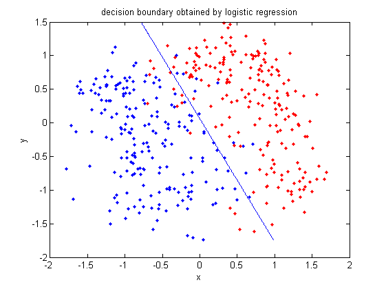
 >>[class, error, POSTERIOR, logp, coeff] = classify(sample, sample, group, 'linear');
 >>k = coeff(1,2).const;
 >>l = coeff(1,2).linear;
 >>f = sprintf('0 = %g+%g*x+%g*y', k, l(1), l(2));
 >>h=ezplot(f, [min(sample(:,1)), max(sample(:,1)), min(sample(:,2)), max(sample(:,2))]);

Plot the decision boundary by LDA. See the previous example for more information about LDA in matlab.

From this figure, we can see that the results of Logistic Regression and LDA are very similar.

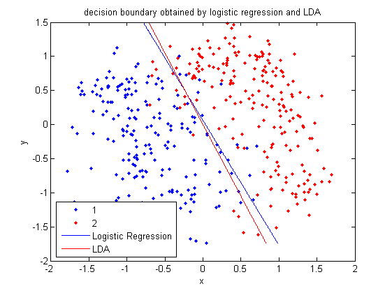
2009.10.21

Multi-Class Logistic Regression

Our earlier goal with logistic regression was to model the posteriors for a 2 class classification problem with a linear function bounded by the interval [0,1]. In that case our model was,

[math]\displaystyle{ \log\left(\frac{P(Y=1|X=x)}{P(Y=0|X=x)}\right)= \log\left(\frac{\frac{\exp(\beta^T x)}{1+\exp(\beta^T x)}}{\frac{1}{1+\exp(\beta^T x)}}\right) =\beta^Tx }[/math]

We can extend this idea to the more general case with K-classes. This model is specified with K - 1 terms where the Kth class in the denominator can be chosen arbitrarily.

[math]\displaystyle{ \log\left(\frac{P(Y=i|X=x)}{P(Y=K|X=x)}\right)=\beta_i^Tx,\quad i \in \{1,\dots,K-1\} }[/math]

The posteriors for each class are given by,

[math]\displaystyle{ P(Y=i|X=x) = \frac{\exp(\beta_i^T x)}{1+\sum_{k=1}^{K-1}\exp(\beta_k^T x)}, \quad i \in \{1,\dots,K-1\} }[/math]

[math]\displaystyle{ P(Y=K|X=x) = \frac{1}{1+\sum_{k=1}^{K-1}\exp(\beta_k^T x)} }[/math]

Note that we still retain the property that the sum of the posteriors is 1. In general the posteriors are no longer complements of each other as in true in the 2 class problem. Fitting a Logistic model for the K>2 class problem isn't as 'nice' as in the 2 class problem since we don't have the same simplification.

The Perceptron

Diagram of a linear perceptron.

Recall the use of Least Squares regression as a classifier,shown to be identical to LDA. To classify points with least squares we take the sign of a linear combination of data points and assign a label equivalent to 1 or -1.

In the 1950s Frank Rosenblatt developed an iterative linear classifier while at Cornell University known as the Perceptron. As in other linear classification methods like Least Squares, Rosenblatt's classifier determines a hyperplane separating the classes.

Particular to the iterative nature of the algorithm, the problem has no global mean(not convex), and does not converge to give a unique hyperplane. If the classes are separable then the algorithm is shown to converge to a local mean. However, for overlapping classes, convergence to a local mean cannot be guaranteed.

As seen in the figure, the perceptron determines the label of the data by computing the sign of a linear combination of components.

Notes

<references/>