stat946w18/Towards Image Understanding From Deep Compression Without Decoding

Paper Title: Towards Image Understanding from Deep Compression Without Decoding - ICLR 2018

Presented By: Aravind Ravi

Introduction

Recent advances in the deep neural network (DNN) based image compression methods have shown potential improvements in image quality, savings in storage and bandwidth reduction. These methods leverage common neural network architectures such as convolutional autoencoders or recurrent neural networks to compress and reconstruct RGB images and outperform classical techniques such as JPEG2000 and BPG on perceptual metrics such as structural similarity index (SSIM) and multi-scale structural similarity index (MS-SSIM).

These approaches encode an image [math]\displaystyle{ x }[/math] to some feature map (compressed representation), which is subsequently quantized to a set of symbols [math]\displaystyle{ z }[/math]. These symbols are then losslessly compressed to a bitstream, from which a decoder reconstructs an image [math]\displaystyle{ {\hat{x}} }[/math], of the same dimensions as [math]\displaystyle{ x }[/math].

Learned compression algorithms have an advantage over engineering compression algorithms in that they can be much more easily adapted to specific domains. For example, a learned compression algorithm might be able to learn good performance on compressing medical images, without specifically tuning the algorithm.

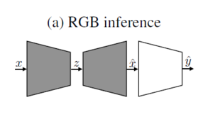
In this paper, the authors explore the idea of applying the learned representations to perform inference without reconstructing the compressed image. Specifically, instead of reconstructing an RGB image from the compressed representation and feeding it to a network for inference, the paper proposes to use a modified network that bypasses reconstruction of the RGB image.

The rationale behind this approach is that the neural network architectures commonly used for learned compression (in particular the encoders) are similar to the ones commonly used for inference, and learned image encoders are hence, in principle, capable of extracting features relevant for inference tasks. The encoder might learn features relevant for inference purely by training on the compression task, and can be forced to learn these features by training on the compression and inference tasks jointly

The advantage of learning an encoder for image compression which produces compressed representation containing features relevant for inference is obvious in scenarios where images are transmitted (e.g. from a mobile device) before processing (e.g. in the cloud), as it saves reconstruction of the RGB image as well as part of the feature extraction and hence speeds up processing. A typical use case is a cloud photo storage application where every image is processed immediately upon upload for indexing and search purposes.

Note: More Information on SSIM, MSSIM

Intuition

Compression techniques (something as common as zipping) are commonly used by us in day to day file handling tasks. Most often we use engineered compression techniques. Deep Neural Networks (DNNs) are nonlinear function approximators which act as feature extractors, extracting features from inputs (like images or sound files). These can be seen as learning based compression techniques as they can perform compression and they can be trained using back propagation as well. If image classification can be done on these compressed files, large image data sets like hyperspectral images and MRI images can be stored efficiently and the compressed files can be used directly by the DNNs for classification or reinforcement learning tasks.

Motivation and Contributions

The authors propose to perform image understanding tasks such as image classification and segmentation directly on DNN based compressed representations. Performing the image understanding tasks on the compressed representations/encoded feature maps has two advantages.

1. This method bypasses the process of decoding the image into the RGB space before classification
2. The authors show that it reduces the overall computational complexity up to 2 times

Contributions of the Paper

• A method to perform image classification and semantic segmentation from compressed representations. In large scale image understanding problems, learning from a compressed representation is definitely something that is interesting.
• The proposed method offers classification accuracy similar to that achieved on decompressed images while reducing the computational complexity by 2 times.
• Semantic segmentation has been shown to be as accurate as performance on decompressed images for moderate compression rates and higher accuracy for aggressive compression rates. In addition, this method achieves lower computational complexity.
• Joint training for image compression and classification has been shown to improve the quality of the image and increase in accuracy of classification and segmentation

Related Work

The prior work has shown image classification from compressed images based on engineered codecs. Some of the works in this area are:

• In video analysis domain: Action recognition (Yeo et al., 2008; Kantorov & Laptev, 2014)
• Classification of compressed hyperspectral images (Hahn et al., 2014; Aghagolzadeh & Radha, 2015)
• Discrete Cosine Transform based compression performed on images before feeding into a neural network, which shows an improvement in training speed by up to 10 times Fu & Guimaraes (2016)
• Video analysis on compressed video (using engineered codecs) has also been studied in the past (Babu et al., 2016)
• Criticism on document image analysis methods (Javed et al.2017)

The authors propose a method that does inference on top of learned feature representation and hence has a direct relation to unsupervised feature learning using autoencoders. They also claim that so far there hasn't been any work using learned compressed representations for image classification and segmentation.

Learned Deeply Compressed Representations

The image compression task is performed based on a convolutional autoencoder architecture proposed by Theis et al. 2017 (shown in the figure below), and a variant of the training procedure described by Agustsson et. al 2017.

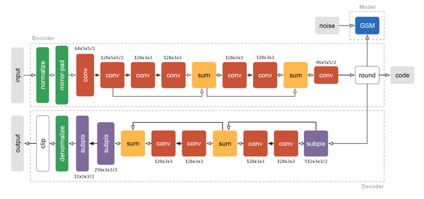
Some points to better understand the architecture:

1. Most convolutions are done in a convolved, lower-dimensional space to speed up computation

2. Different activation functions are used. Blank arrows indicate the identity function (no additional linearity), while black arrows indicate leaky rectifications

3. The “round” box simply rounds all elements in the tensor to the nearest integer

4. The “subpix” block is just an upsampling /reconstruction block where the feature map’s coefficients are reshuffled after a convolution

Compression Architecture

The compression network is an autoencoder that takes an input image [math]\displaystyle{ x }[/math] and outputs [math]\displaystyle{ {\hat{x}} }[/math] as the approximation to the input.

The encoder has the following structure: It starts with 2 convolutional layers with spatial subsampling by a factor of 2, followed by 3 residual units, and a final convolutional layer with spatial subsampling by a factor of 2. This results in a [math]\displaystyle{ w/8 }[/math] x [math]\displaystyle{ h/8 }[/math] x [math]\displaystyle{ C }[/math] dimensional representation, where [math]\displaystyle{ w }[/math] and [math]\displaystyle{ h }[/math] are the spatial dimensions of [math]\displaystyle{ x }[/math], and the number of channels C is a hyperparameter related to the rate [math]\displaystyle{ R }[/math]. This representation is then quantized to a discrete set of symbols, forming a compressed representation, [math]\displaystyle{ z }[/math].

To get the reconstruction [math]\displaystyle{ {\hat{x}} }[/math], the compressed representation is fed into the decoder, which mirrors the encoder, but uses upsampling and deconvolutions instead of subsampling and convolutions.

Quantizing the compressed representation imposes a distortion [math]\displaystyle{ D }[/math] on [math]\displaystyle{ {\hat{x}} }[/math] w.r.t. [math]\displaystyle{ x }[/math], i.e., it increases the reconstruction error. This is traded for a decrease in entropy of the quantized compressed representation [math]\displaystyle{ z }[/math] which leads to a decrease of the length of the bitstream as measured by the rate [math]\displaystyle{ R }[/math]. Thus, to train the image compression network, the classical rate-distortion trade-off [math]\displaystyle{ D + \beta R }[/math] is minimized. As a metric for [math]\displaystyle{ D }[/math], the mean squared error (MSE) between [math]\displaystyle{ x }[/math] and [math]\displaystyle{ {\hat{x}} }[/math] are used and [math]\displaystyle{ R }[/math] is estimated using [math]\displaystyle{ H(q) }[/math]. [math]\displaystyle{ H(q) }[/math] is the entropy of the probability distribution over the symbols and is estimated using a histogram of the probability distribution (as done by Agustsson et al., 2017). The trade-off between MSE and the entropy is controlled by adjusting [math]\displaystyle{ \beta }[/math]. For each [math]\displaystyle{ \beta }[/math] an operating point is derived where the images have a certain bit rate, as measured by bits per pixel (bpp), and corresponding MSE. To better control the bpp, a target entropy Ht is introduced by the authors to formulate the loss defined as:

\begin{align} \mathcal{L_c} = \text{MSE}(x,{\hat{x}})+\beta\max({H(q)}-{H_t},0) \end{align}

Agustsson et. al 2017, proposed a method to overcome the issue of non-differentiability of the quantization step by proposing a differentiable approximation to the quantization. This method has been adapted to suit the current application in the paper.

Three operating points at 0.0983 bpp (C=8), 0.330 bpp (C=16), and 0.635 bpp (C=32) are obtained empirically. All further experiments are performed with these three operating points and the results for the same are presented in the following sections.

Image Classification from Compressed Representations

Classification on RGB Images

For the image classification task based on the RGB images, the authors use the ResNet-50 architecture. Further information on residual networks can be found in the following links: ResNets Part-1 ResNets Part-2

The details of the architecture are presented in the table below:

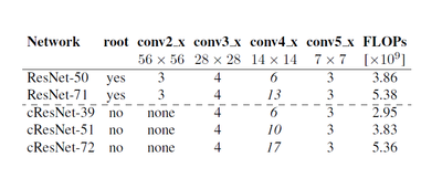
In this paper, the number of 14x14 (conv4_x) blocks have been modified to obtain a new architecture called ResNet-71.

Classification on Compressed Representations

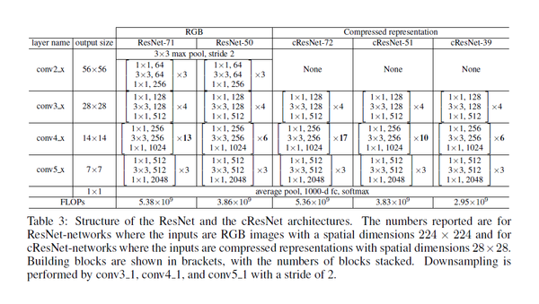
For input images with spatial dimension 224x224, the encoder of the compression network outputs a compressed representation with dimensions 28x28xC, where C is the number of channels. To use this compressed representation as input to the classification network, a simple variant of the ResNet architecture is proposed. This variant is referred to as cResNet-k, where c stands for “compressed representation” and k is the number of convolutional layers in the network. These networks are constructed by simply “cutting off” the front of the regular (RGB) ResNet. The root-block of the network and the residual layers that have a larger spatial dimension than 28x28 are removed. To adjust the number of layers k, the ResNet architecture proposed by He et al. (2015) is used and the number of 14x14 (conv4 x) residual blocks are modified.

In this way, three different architectures are derived:

• cResNet-39 is ResNet-50 with the first 11 layers removed as described above, and this significantly reduces computational cost
• cResNet-51
• cResNet-72

cResNet-51 and cResNet-72 are obtained by adding 14x14 residual blocks to match the computational cost of ResNet-50 and ResNet-71 respectively.

The detailed description of all the network architectures are presented below:

Semantic Segmentation from Compressed Representations

For semantic segmentation, the ResNet based DeepLab architecture is adapted for the proposed application. The cResNet and ResNet image classification architectures are re-purposed with atrous convolutions, where the filters are upsampled instead of downsampling the feature maps. This is done to increase their receptive field and to prevent aggressive subsampling of the feature maps. For segmentation, the ResNet architecture is restructured such that the output feature map has 8 times smaller spatial dimension than the original RGB image (instead subsampling by a factor 32 times like for classification). When using the cResNets the output feature map has the same spatial dimensions as the input compressed representation (instead of subsampling 4 times like for classification). This results in comparably sized feature maps for both the compressed representation and the reconstructed RGB images. Finally the last 1000-way classification layer of these classification architectures is replaced by an atrous spatial pyramid pooling (ASPP) with four parallel branches with rates {6, 12, 18, 24}, which provides the final pixel-wise classification.

Joint Training for Compression and Image Classification

The authors propose a joint training strategy to combine compression and classification tasks. To do this, the proposed method combines the compression network and the cResNet-51 architecture. The figure below shows the combined pipeline:

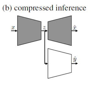
All parts, encoder, decoder, and inference network, are trained at the same time. The compressed representation is fed to the decoder to optimize for mean-squared reconstruction error and to a cResNet-51 network to optimize for classification using a cross-entropy loss. The combined loss function takes the form:

\begin{align} \mathcal{L_c} = \gamma(\text{MSE}(x,{\hat{x}})+\beta\max({H(q)}-{H_t},0))+l_{ce}(y,{\hat{y}}) \end{align}

where the loss terms for the compression network, [math]\displaystyle{ \mathcal{L_c} = \text{MSE}(x,{\hat{x}})+\beta\max({H(q)}-{H_t},0) }[/math], are the same as in training for compression only. [math]\displaystyle{ l_{ce} }[/math] is the cross-entropy loss for classification. [math]\displaystyle{ \gamma }[/math] controls the trade-off between the compression loss and the classification loss.

Experiments and Results

Learned Deeply Compressed Representations Results

All experiments have been performed on the ILSVRC2012 dataset.

The metrics used to measure the compression quality are as follows:

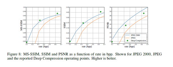
• PSNR (Peak Signal-to-Noise Ratio) is a standard measure, depending monotonically on mean squared error defined as:

\begin{align} PSNR = 10(\log_{10}(255^2/MSE)) \end{align}

• SSIM (Structural Similarity Index) and MS-SSIM (Multi-Scale SSIM) are metrics proposed to measure the similarity of images as perceived by humans

The figure below depicts the performance of the deep compression models vs. standard JPEG and JPEG2000. Higher values are better. The proposed technique outperforms the JPEG and JPEC2000 at the operating points used in this paper.

The learned compressed representations are illustrated in the figure below.

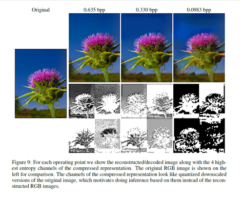
In the above figure, the original RGB-image is shown along with compressed versions of the RGB image which are reconstructed from the compressed representations. The 4 channels with the highest entropy are shown in the visualizations. These visualizations indicate how the networks compress an image, as the rate (bpp) gets lower the entropy cost of the network forces the compressed representation to use fewer quantization levels, as can clearly be seen. For the most aggressive compression, the channel maps use only 2 levels for the compressed representation.

Classification on Compressed Representations

All experiments have been performed on the ILSVRC2012 dataset. It consists of 1.28 million training images and 50k validation images. These images are distributed across 1000 diverse classes. For image classification, the top-1 classification accuracy and top-5 classification accuracy are reported on the validation set on 224x224 center crops for RGB images and 28x28 center crops for the compressed representation.

Training Procedure

The compression network is fixed while training the classification network, both when training with compressed representations and with reconstructed compressed RGB images. For the compressed representations, the output of the fixed encoder (the compressed representation) is provided input to the cResNets (decoder is not needed). When training on the reconstructed compressed RGB images, the output of the fixed encoder-decoder (RGB image) is provided as input to the ResNet. This is done for each operating point.

Refer to Appendix A Section A4, of the paper for details on the hyperparameters and optimization used for training the network [1].

Classification Results

The tables below present the results of the classification at each operating point, both classifying from the compressed representation and the corresponding reconstructed compressed RGB images.

400

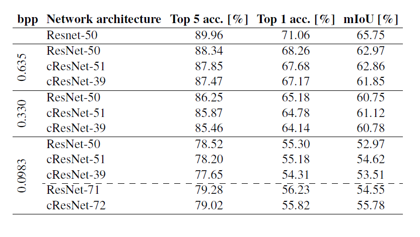
Figure below shows the validation curves for ResNet-50, cResNet-51, and cResNet-39.

700

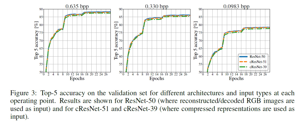
For the 2 classification architectures with the same computational complexity (ResNet-50 and cResNet-51), the validation curves at the 0.635 bpp compression operating point almost coincide, with ResNet-50 performing slightly better. As the rate (bpp) gets smaller this performance gap gets smaller. The table above shows the classification results when the different architectures have converged. At the 0.635 bpp operating point, ResNet-50 only performs 0.5% better in top-5 accuracy than cResNet-51, while for the 0.0983 bpp operating point this difference is only 0.3%. Using the same pre-processing and the same learning rate schedule but starting from the original uncompressed RGB images yields 89.96% top-5 accuracy. The top-5 accuracy obtained from the compressed representation at the 0.635 bpp compression operating point, 87.85%, is even competitive with that obtained for the original images at a significantly lower storage cost. Specifically, at 0.635 bpp the ImageNet dataset requires 24.8 GB of storage space instead of 144 GB for the original version, a reduction by a factor 5.8 times.

Notes on top-1 and top-5 accuracy:

• Top-1 accuracy: This is the conventional accuracy metric used in machine learning. Wherein if the true label of the input to a model matches the highest probability class of the last layer of the output of CNN (predicted class probability), then the given input is correctly classified, else it is considered as incorrectly classified.
• Top-5 accuracy: In this case, if any of the model's 5 highest classification probabilities match with the true label of the input, then this is considered as a correct classification, else it is an incorrect classification.

Semantic Segmentation Results

All experiments have been performed on the PASCAL VOC-2012 dataset for semantic segmentation. It has 20 object foreground classes and 1 background class. The dataset consists of 1464 training and 1449 validation images. In every image, each pixel is annotated with one of the 20 + 1 classes. The original dataset is furthermore augmented with extra annotations, so the final dataset has 10,582 images for training and 1449 images for validation.

All performance is measured on pixel wise intersection-over-union (IoU) averaged over all the classes or mean-intersection-over-union (mIoU) on the validation set.

Details on IoU

Training Procedure

The cResNet/ResNet networks are pre-trained on the ImageNet dataset using the procedure described earlier on the image classification task, the encoder and decoder is fixed as in the earlier scenario. The architectures are then adapted with dilated convolutions, cResNet-d/ResNet-d, and finetuned on the semantic segmentation task.

Refer to Appendix A Section A5, of the paper for details on the hyperparameters and optimization used for training the network [1].

Segmentation Results

The table below shows the mIoU results for the segmentation task.

450

The figure below illustrates the segmentation results with respect to each compression operating point.

700

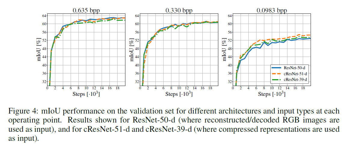
For semantic segmentation ResNet-50-d and cResNet-51-d perform equally well at the 0.635 bpp compression operating point. For the 0.330 bpp operating point, segmentation from the compressed representation performs slightly better, 0.37%, and at the 0.0983 bpp operating point segmentation from the compressed representation performs considerably better than for the reconstructed compressed RGB images, by 1.65%.

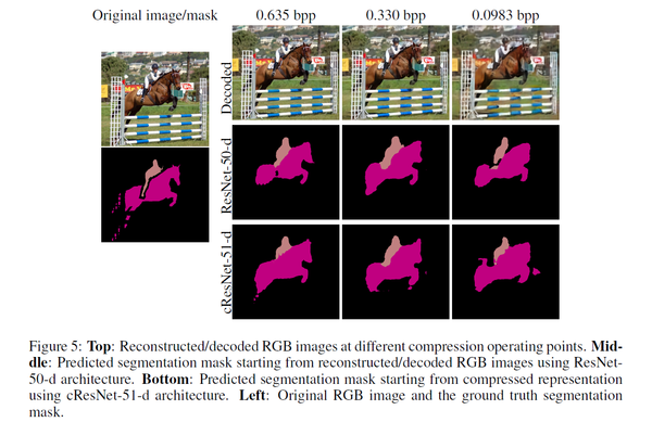
The above figure shows the predicted segmentation visually for both the cResNet-51-d and the ResNet-50-d architecture at each operating point. Along with the segmentation, it also shows the original uncompressed RGB image and the reconstructed compressed RGB image. These images highlight the challenging nature of these segmentation tasks, but they can nevertheless be performed using the compressed representation. They also clearly indicate that the compression affects the segmentation, as lowering the rate (bpp) progressively removes details in the image. Comparing the segmentation from the reconstructed RGB images to the segmentation from the compressed representation visually, the performance is similar.

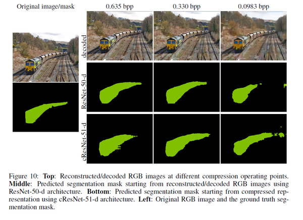
The figure below is another example of visual results of segmentation from compressed representation and reconstructed RGB images. The performance is visually similar for all operating points except for the 0.0983 bpp operating point where the reconstructed RGB image fails to capture the back part of the train, while the compressed representation manages to capture that aspect of the image in the segmentation.

Results on Computational Gains

Computational Gains on Classification

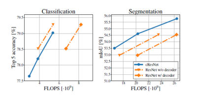
The figure on the left illustrates, the top-5 classification accuracy as a function of computational complexity for the 0.0983 bpp compression operating point. Looking at a fixed computational cost, the reconstructed compressed RGB images perform about 0.25% better. Looking at a fixed classification cost, inference from the compressed representation costs about 0.6 * 10^9 FLOPs more. However when accounting for the decoding cost at a fixed classification performance, inference from the reconstructed compressed RGB images costs 2.2*10^9 FLOPs more than inference from the compressed representation.

Computational Gains on Segmentation

In the figure on the right illustrates, the mIoU validation performance is shown as a function of computational complexity for the 0.0983 bpp compression operating point. Here, even without accounting for the decoding cost of the reconstructed images, the compressed representation performs better. At a fixed computational cost, segmentation from the compressed representation gives about 0.7% better mIoU. And at a fixed mIoU the computational cost is about 3.3*10^9 FLOPs lower for compressed representations. Accounting for the decoding costs this difference becomes 6.1*10^9 FLOPs. due to the nature of the dilated convolutions and the increased feature map size, the relative computational gains for segmentation are not as pronounced as for classification.

Joint Training for Compression and Image Classification

Training Procedure

When doing joint training, the compression network and the classification networks are first initialized from a trained state obtained as described previously. After initialization, the networks are both finetuned jointly. For a detailed description of hyperparameters used and the training schedule see Appendix A8.

To control that the change in classification accuracy is not only due to (1) a better compression operating point or (2) the fact that the cResNet is trained longer, the following is done. A new operating point is obtained by finetuning the compression network only using the schedule described above. The cResNet-51 is trained on top of this new operating point from scratch. Finally, the compression network is fixed at the new operating point, and the cResNet-51 is trained for 9 epochs.

To obtain segmentation results, the jointly trained network is used. The operating point is fixed and the jointly finetuned classification network is adopted fro segmentation (cResNet-51-d).

Joint Training Results

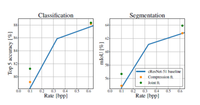
It can be seen from the figure, that the classification and segmentation results “move up” from the baseline through fine tuning. When training jointly the improvement for classification are larger and a significant improvement for segmentation is achieved. For the 0.635 bpp operating point the classification performance is similar for training the network jointly and training the compression network only, but when using these operating points for segmentation the difference is considerable.

The results presented by the authors suggest an improvement in classification by 2%, a performance gain which would require an additional 75% of the computational complexity of cResNet-51. The segmentation performance after training the networks jointly is 1.7% better in mIoU than training only the compression network.

Critique

The paper proposes how previous work in auto-encoders and image compression can be extended effectively to a novel task of a combined image compression and recognition task. The work has provided extensive experimental evaluation and evidence that suggests that learned compressed representations can be effective in classification and segmentation tasks. While maintaining the performance of the techniques to state of the art performance, the authors show that the proposed method can offer significant computational gains. The applications of this can be in multimedia communication, wireless transmission of images, video surveillance on the mobile edge, etc. With the advent of 5G and other new wireless technologies, this method offers capabilities that can be utilized to conserve wireless bandwidth, savings on storage while retaining the perceptual quality of images. The joint training of compression and classification network provides some added advantages and also shows that at aggressive compression rates the performance in classification and segmentation can be improved significantly.

Another critique is the authors did not answer the question of why we want to do image understanding from a compressed space. From the intuitive sense, the learning algorithm could easily just learn from the original feature space, which obviously contains more information. The troubling part is that the author does not answer a more fundamental question of why learning from a compressed space would bring any benefit compared to learning directly from the original feature space.

The authors mention that the complexity of the current approach is still high in comparison with methods like JPEG or JPEG2000. They also mention that this can be overcome when the networks are trained and run on GPU's. Although this has been seen as a drawback, with subsequent improvements in physical hardware and more specialized deep learning platforms, the limitation of the current approach can be overcome. While the authors did thorough experiments and gave extensive results on compressed representations and their advantages, the idea itself is not very novel.Finally, in the light of providing extensive experimental contributions, the authors have written a quite lengthy paper. There are parts of the paper where the ideas have been repeated frequently, and this could've been avoided leading to a more well-balanced length of the article.

• ([[1]]) As it is mentioned in the paper, solving a Vision problem directly from a compressed image, is not a novel method (e.g: DCT coefficients were used for both vision and audio data to solve a task without any decompression).

Conclusion

The paper proposes an inference task using compressed image representations without the need to decode for classification and semantic segmentation. The paper has successfully demonstrated through a set of rigorous experiments the approach for performing the intended tasks. The results show significant improvements in computational complexity while maintaining state of the art classification and segmentation performance. The authors also intend to explore other computer vision tasks based on using compressed representation as part of the future work. They also suggest that this could potentially lead to gaining a better understanding of the features/compressed representations learned by image compression networks leading to applications in unsupervised or semi-supervised learning.

References

1. Torfason, R., Mentzer, F., Agustsson, E., Tschannen, M., Timofte, R., & Van Gool, L. (2018). Towards image understanding from deep compression without decoding. arXiv preprint arXiv:1803.06131.
2. Theis, L., Shi, W., Cunningham, A., & Huszár, F. (2017). Lossy image compression with compressive autoencoders. arXiv preprint arXiv:1703.00395.
3. Agustsson, E., Mentzer, F., Tschannen, M., Cavigelli, L., Timofte, R., Benini, L., & Gool, L. V. (2017). Soft-to-hard vector quantization for end-to-end learning compressible representations. In Advances in Neural Information Processing Systems (pp. 1141-1151).
4. He, K., Zhang, X., Ren, S., & Sun, J. (2016). Deep residual learning for image recognition. In Proceedings of the IEEE conference on computer vision and pattern recognition (pp. 770-778).
5. Chen, L. C., Papandreou, G., Kokkinos, I., Murphy, K., & Yuille, A. L. (2018). Deeplab: Semantic image segmentation with deep convolutional nets, atrous convolution, and fully connected crfs. IEEE transactions on pattern analysis and machine intelligence, 40(4), 834-848.