Towards Deep Learning Models Resistant to Adversarial Attacks

This is a summary of the paper "Towards Deep Learning Models Resistant to Adversarial Attacks" by Aleksander Madry, Aleksandar Makelov, Ludwig Schmidt, Dimitris Tsipras, and Adrian Vladu. ^[1]

Presented by

• Yongqi Dong
• Aden Grant
• Andrew McMurray
• Jameson Ngo
• Baizhi Song
• Yu Hao Wang
• Amy Xu

1. Introduction

Figure 1. Before and after an input image of a panda was subjected to perturbations.^Source

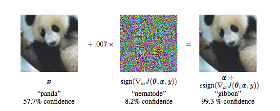
Any classifier can be tricked into giving the incorrect result. When an input is specifically designed to do this, it is called an adversarial attack. This can be done by injecting a set of perturbations to the input. These attacks are a prominent challenge for classifiers that are used for image processing and security systems because small changes to the input values that are imperceptible to the human eye can easily fool high-level neural networks. As such, resistance to adversarial attacks has become increasingly important for classifiers to have.

While there have been many approaches to defend against adversarial attacks, we can never be certain that these defenses will be able to robust against broad types of adversaries. Furthermore, these defenses can be evaded by stronger and adaptive adversaries.

Contributions

This paper uses robust optimization to explore adversarial robustness of neural networks. The authors conduct an experimental study of the saddle-point formulation which is used for adversarially training. The authors propose that we can reliably solve the saddle-point optimization problem using first-order methods, particularly project gradient descent and stochastic gradient descent, despite the problem's non-convexity and non-concavity. They explore how network capacity affects adversarial robustness and conclude that networks need larger capacity in order to be resistant to strong adversaries. Lastly, they train adversarially robust networks on MNIST and CIFAR10 using the saddle point formulation.

2. An Optimization View on Adversarial Robustness

Consider a standard classification task on data [math]\displaystyle{ x \in \mathbb{R}^d }[/math] and labels [math]\displaystyle{ y \in [1,...,k] }[/math], assumed to have underlying distribution [math]\displaystyle{ D }[/math]. Based a given loss function [math]\displaystyle{ L(\theta,x,y) }[/math] (e.g. the cross-entropy loss), the goal is to find the model parameters [math]\displaystyle{ \theta \in \mathbb{R}^p }[/math] that minimize the empirical risk of misclassification. In other words, the problem is to solve:

[math]\displaystyle{ \min_{\theta} \mathbb{E}_{(x,y) \sim D} [L(\theta,x,y)] }[/math]

However, empirical risk minimization may not result in models that are robust against adversaries. To produce robust models, we instead define conditions that the model must satisfy and train the model according to those conditions. We describe the set of attacks that our model must be robust against by considering a set of perturbations [math]\displaystyle{ S \subseteq \mathbb{R}^d }[/math] for each data point [math]\displaystyle{ x }[/math]. This gives a set of data points with similar properties to [math]\displaystyle{ x }[/math], for example, the [math]\displaystyle{ l_{\infty} }[/math]-ball around [math]\displaystyle{ x }[/math], which we focus on in this paper.

We then define an augmented classification algorithm based on perturbed input data rather than the natural data. Our goal then becomes finding the model parameters [math]\displaystyle{ \theta \in \mathbb{R}^p }[/math] which minimize the expected loss calculated on perturbed data. This results in a saddle point problem:

[math]\displaystyle{ \min_{\theta} \mathbb{E}_{(x,y) \sim D} [\max_{\delta \in S} L(\theta,x+\delta,y)] }[/math]

We rewrite this as [math]\displaystyle{ \min_{\theta} \rho (\theta) }[/math] where [math]\displaystyle{ \rho (\theta) }[/math] is the adversarial loss of the network; this problem thus becomes the primary topic of this paper. The saddle point problem has two components:

1. Inner maximization: [math]\displaystyle{ \qquad \max_{\delta \in S} L(\theta,x+\delta,y) }[/math]
   This involves finding the adversarial version of input data [math]\displaystyle{ x }[/math] that results the highest loss, which is equivalent to building an attack against the network.
2. Outer minimization: [math]\displaystyle{ \qquad \min_{\theta} \rho (\theta) }[/math]
   This involves finding model parameters that minimize the above adversarial loss, i.e. training the network to be adversarially robust.

3. Adversarially Robust Networks

Obtaining the outer minimization of the saddle point formulation [math]\displaystyle{ \min_{\theta} \rho (\theta) }[/math] guarantees that all perturbations result in smallest adversarial loss possible based on the attack. Stochastic gradient descent (SGD) is used to solve the outer minimization problem by obtaining the gradients [math]\displaystyle{ \nabla_\theta \rho(\theta) }[/math], which are computed at the maximizer of the inner maximization problem.

Solutions for the inner maximization are used as known adversarial attacks on the neural network.

Inner maximization

Based on prior research, the maximizers [math]\displaystyle{ \delta \in S }[/math] of [math]\displaystyle{ \rho(\delta) }[/math] are obtained by using projected gradient descent (PGD). Since the inner maximization is non-concave, the global maximizer cannot be found using PGD (instead, PGD will converge to local maxima). However, the paper’s findings conclude that PGD can be used in practice to solve the inner maximization problem using first-order methods.

Applying Danskin’s theorem on a subset [math]\displaystyle{ S' \in S }[/math] where the local maximum is the global maximum of the region [math]\displaystyle{ S' }[/math] gives the gradient corresponding to the descent direction for the saddle point problem when the adversary is constrained to [math]\displaystyle{ S' }[/math]. The authors also find that the local maxima are widely spread apart within [math]\displaystyle{ x_i+S }[/math] and tens to have similar loss values for both normally and adversarially trained networks.

Figure 2. Adversarial loss of MNIST and CIFAR10 from 20 runs of PGD starting at random points in the [math]\displaystyle{ \ell_\infty }[/math]-ball around the same benign example.

Outer minimization

Since distribution [math]\displaystyle{ D }[/math] is unknown, the gradients and [math]\displaystyle{ \rho(\theta) }[/math] are obtained using sampled input points, i.e. for the case of a single random example [math]\displaystyle{ x }[/math] with label [math]\displaystyle{ y }[/math], the problem becomes:

[math]\displaystyle{ \min_\theta [max_{\delta \in S} L(\theta, x+\delta,y)] }[/math]

[math]\displaystyle{ L }[/math] is assumed to be continuously differentiable for [math]\displaystyle{ \theta }[/math], and Danskin’s theorem is used to obtained the direction of descent. Discontinuity when using ReLU activations is assumed to not be an issue as the set of discontinuities has a measure of zero, and thus these points of discontinuity will never be encountered. Using the gradients [math]\displaystyle{ \nabla_\theta \rho(\theta) }[/math] obtained with SGD, the loss of the saddle point problem is reduced during training. Thus, the saddle point optimization problem can be solved and classifiers can be trained to be adversarially robust.

4. Experiments

Training

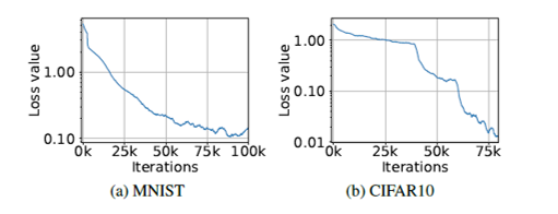
We put into practice our robust classification framework with the MNIST and CIFAR10 datasets, with a projected gradient descent (PGD) training adversary, chosen because it effectively produces almost-maximal loss. We start PGD at a randomly chosen perturbation of the natural data. For both datasets, we see a sustained decrease in training loss when networks are trained against the PGD adversary, which suggests that adversarial loss is effectively being minimized.

Figure 3. Trajectory of cross-entropy loss when training with a projected gradient descent (PGD) adversary.

Testing

The trained models are then tested based on a variety of adversaries.

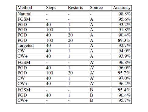
The source networks for the adversarial attacks are:

• the network itself, denoted by source A (white-box attacks).
• an independently trained version of the original network, denoted by source A' (black-box attacks).
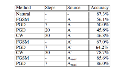
• a version of the original network trained on natural data only, denoted by Anat (black-box attacks).
• a network with a different convolutional architecture, as described by Tramèr et al. (2017), denoted by B (black-box attacks).

The attack methods used are:

• Fast Gradient Sign Method (denoted FGSM)
• Projected gradient descent (denoted PGD) with various steps and restarts
• Attacks based on literature by Carlini & Wagner (2016b), denoted by CW; a version of this attack with a high confidence parameter is denoted by CW+

MNIST: Network structure and results

For the MNIST model, the network is composed of two convolutional layers (with 32 and 64 filters) and a fully connected 1024-unit layer. Each convolutional layer is followed by [math]\displaystyle{ 2 \times 2 }[/math] max-pooling layers. The training adversary used is PGD with 40 steps and a step size of 0.01 in the [math]\displaystyle{ l_\infty }[/math]-norm, with perturbation size [math]\displaystyle{ \varepsilon=0.3 }[/math]. The adversarially trained model was evaluated to be highly robust; testing results are given in Table 1.

Table 1. MNIST dataset: Adversarially-trained network performance against various adversaries with [math]\displaystyle{ \varepsilon=0.3 }[/math]; most successful attacks are bolded for each attack model.

CIFAR10: Network structure and results

For the CIFAR10 model, the network architectures used are the Resnet model (as per He et al (2016); TFM (2017)) and a version of Resnet with [math]\displaystyle{ 10 \times }[/math] wider layers. The training adversary is PGD with 7 steps and a step size of 2 in the [math]\displaystyle{ l_\infty }[/math]-norm, with perturbation size [math]\displaystyle{ \varepsilon=8 }[/math] total. The most challenging testing adversary (white-box PGD) used the same architecture as above with 20 steps. Th adversarially trained model performed well given the strength of the testing adversaries but struggled in some cases, with test accuracy close to or lower than 50%. Testing results are given in Table 2.

Table 2. CIFAR10 dataset: Adversarially-trained network performance against various adversaries with [math]\displaystyle{ \varepsilon=8 }[/math]; most successful attacks are bolded for each attack model.

Further experiments: [math]\displaystyle{ \varepsilon }[/math] values and [math]\displaystyle{ l_2 }[/math]-bounded attacks

The MNIST model adversarially trained against [math]\displaystyle{ l_\infty }[/math]-bounded attacks with [math]\displaystyle{ \varepsilon = 0.3 }[/math] and the CIFAR10 model trained against [math]\displaystyle{ l_\infty }[/math]-bounded attacks with [math]\displaystyle{ \varepsilon = 8 }[/math] are further evaluated against attacks of varying [math]\displaystyle{ \varepsilon }[/math] values, for both [math]\displaystyle{ l_\infty }[/math]-bounded and [math]\displaystyle{ l_2 }[/math]-bounded attacks. The MNIST network performed especially well against [math]\displaystyle{ l_2 }[/math]-bounded adversaries.

Figure 4. Adversarially-trained MNIST and CIFAR10 network performance tested against PGD adversaries of varying [math]\displaystyle{ \varepsilon }[/math] values, for [math]\displaystyle{ l_\infty }[/math] and [math]\displaystyle{ l_2 }[/math] norms. [math]\displaystyle{ \varepsilon }[/math] value used for training is indicated in red.

Training accuracy

The MNIST network and wide-layer version of the CIFAR10 network had 100% accuracy on the training sets; thus, the optimization problem is tractable.

Running time

As PGD is iterative, training against a [math]\displaystyle{ k }[/math]-step PGD adversary requires [math]\displaystyle{ k }[/math] forward and backward passes per training batch rather than the single forward and backward pass for standard network training. This poses a challenge for computation as the the running time is greater by a factor of [math]\displaystyle{ k+1 }[/math].

5. First-Order Adversaries

Since all local maxima founded by PGD tended to have similar loss values, it is unlikely that any other first-order adversary will yield a local maxima with a significantly lower final loss value than the PGD adversary. This is seen experimentally: other adversaries with significantly lower loss values are not found even after a large amount of restarts.

The authors also experimentally find that a network trained to be robust against PGD adversaries also become robust against various other first-order adversaries. This result, along with the fact that the vast majority of optimization problems in machine learning are solved using first-order methods, suggest that using the saddle point formulation to adversarially train networks will encompass all current approaches that attempt to achieve adversarial robustness.

Transfer attacks

Transfer attacks are adversarial attacks that do not have direct access to the classifier. Although these attacks evaluate the classifier without the gradient, it can be estimated with finite differences. Thus, first-order attacks are relevant and are use to train against these attacks. The paper finds that increasing network capacity and the strength of the adversary that the network is trained against improves resistance to transfer attacks. The paper also finds that the models that are resistant to first-order attacks are more resistant to transfer attacks.

6. Conclusions

Neural Networks can be made resistant to adversarial attacks. We can design reliable adversarial training methods through a surprisingly regularly structured saddle point optimization problem. Even though the overall problem relates to a maximization of a non-concave function with varying maxima, these maxia are highly concentrated. Truly robust accurate adversarial models are possible after further exploration.

References

• ^[1] Aleksander Madry, Aleksandar Makelov, Ludwig Schmidt, Dimitris Tsipras, and Adrian Vladu. Towards Deep Learning Models Resistant to Adversarial Attacks. In Proceedings of the ICLR 2018 Conference, Vancouver, BC.
• ^[2] Carlini, N., Wagner, D. (2016). Defensive distillation is not robust to adversarial examples. arXiv preprint arXiv:1607.04311.
• ^[3] Carlini, N., Wagner, D. (2017). Towards evaluating the robustness of neural networks. In 2017 IEEE Symposium on Security and Privacy (SP) (pp. 39-57). IEEE.
• ^[4] He, K., Zhang, X., Ren, S., Sun, J. (2016). Deep residual learning for image recognition. In Proceedings of the IEEE conference on computer vision and pattern recognition (pp. 770-778).
• ^[5] Tramèr, F., Kurakin, A., Papernot, N., Goodfellow, I., Boneh, D., McDaniel, P. (2017). Ensemble adversarial training: Attacks and defenses. arXiv preprint arXiv:1705.07204.
• ^[6] Ian J. Goodfellow, Jonathon Shlens, and Christian Szegedy. (2014). Explaining and harnessing adversarial examples. arXiv preprint arXiv:1412.6572.
• ^[7] Tensor flow models repository. https://github.com/tensorflow/models/tree/master/resnet, 2017.