Representations of Words and Phrases and their Compositionality

Representations of Words and Phrases and their Compositionality is a popular paper published by the Google team led by Tomas Mikolov in 2013. It is known for its impact in the field of Natural Language Processing and the techniques described below are still used today.

Presented by

• F. Jiang
• J. Hu
• Y. Zhang

Introduction

This paper, "Distributed Representations of Words and Phrases and their Compositionality" proposes several methods of improving the performance metrics of the Skip-gram model introduced in a previous paper, a Natural Language Processing technique of encoding words as arbitrary dimensional vectors using a neural network framework. Notably, the Skip-gram model can be made to train faster and produce higher accuracy via a number of simple adjustments; the replacement of the hierarchical soft max function with simple negative sampling, and the subsampling of frequent words.

Skip Gram Model

The Skip-gram model is a Natural Language Processing method based upon a neural network structure designed to learn vector representations of words in such a way as to produce similar encodings for words that appear in similar contexts. While the model can be used to evaluate certain probabilities, this is considered a side effect of its learning process; its primary function is that of a Word2Vec encoder.

Skip-gram is structured as a one-layer neural network with no non-linear activation function in the hidden layer but a soft-max classifier in the output layer. Words or phrases are encoded using one-hot encoding; the input and output vectors are constructed such that the index of a certain word is indicated by the number 1 within a length determined by a pre-specified vocabulary or corpus (e.g. the word "ant" indicated by 1 at its position in the corpus vector while everything else is 0). The size of the hidden layer is also specified as a hyper parameter; larger sizes of the hidden layer will result in encodings of better quality but take longer to train.

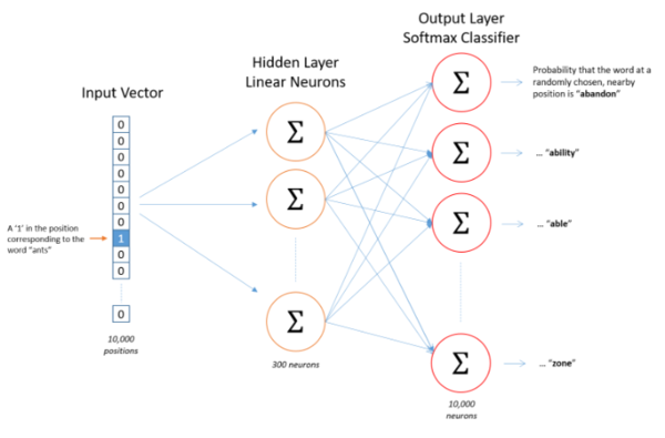
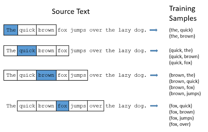
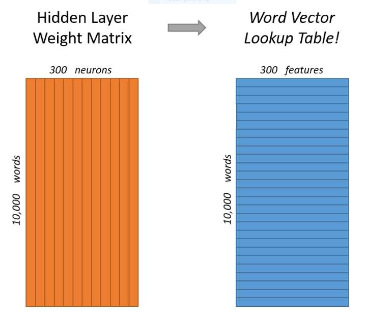
The central premise behind Skip-gram's learning process is that words or phrases that appear close together regularly in the training set are deemed to have similar contexts and should therefore be encoded in such a way as to maximize the probability of the model predicting their appearance together. Training data is prepared by producing a series of word pairs from the training test via a "window size" hyper-parameter that specifies all words a certain number ahead and behind the target word as the desired output, while iterating through all the words of the passage. For example, the model will may learn from the training set that "steering" and "wheel" appear in similar contexts. This means that one is a good predictor of the other, but also that "driving" is a good predictor of both. Thus, feeding any one of them into the model should produce high probabilities (of each appearing in the same context) for the all the others. Once we have a neural net that predicts contextual probabilities to an acceptable degree, the hidden layer weights are saved as the desired Word2Vec encodings (as an nxd matrix, each row represents a single encoding for the corpus word at that row index)

One advantage of the Skip-gram model over older N-gram models is that the encodings preserve certain linguistic patterns that manifest in surprisingly clear and intuitive ways. For example, linear operations work on skip-gram encodings in a surprisingly logical way; the paper notes that on their trained model, vec(“Madrid”) - vec(“Spain”) + vec(“France”) is closer to vec(“Paris”) than to any other word vector in the corpus. In a sense, subtracting "Spain" from "Madrid" extracts the notion of a capital city that when added to "France", produces "Paris". This property is so attractive that the paper uses it as a benchmark for their Skip-gram implementations ("Do linear operations produce logical results?")

Hierarchical Softmax

Although the Skip-gram method is described using the soft-max function [math]\displaystyle{ (1) }[/math] for the purposes of computing [math]\displaystyle{ \nabla \log p(w_{O}|w_{I}) }[/math] for the backpropagation stages, practical considerations make it difficult to calculate this gradient, particularly if the corpus contains many words since it computational complexity scales linearly with [math]\displaystyle{ W }[/math]

[math]\displaystyle{ (1)\quad p(w_{O}|w_{I}) = \frac{exp(v_{w_{O}}^{'T}v_{w_{I}})}{\sum_{w=1}^W exp(v_{w_{O}}^{'T}v_{w_{I}})} }[/math] where [math]\displaystyle{ v_{w} }[/math] and [math]\displaystyle{ v_{w}' }[/math] are the input and output representations of [math]\displaystyle{ w }[/math] and [math]\displaystyle{ W }[/math] is the vocabulary size

Instead, the Skip-gram model described in Mikolov et al. used an approximation called Hierarchical softmax which provides better asymptotic performance for large numbers of output nodes. Rather than evaluate W output nodes, hierarchical soft-max can instead evaluate [math]\displaystyle{ \log W }[/math] nodes. This is done by encoding the output layer using a binary or Huffman tree where the [math]\displaystyle{ W }[/math] words are represented as leaves and each node represents the relative probability of all its child nodes. Optimal asymptotic performance can be achieved if the tree is a balanced binary tree, in which case [math]\displaystyle{ \log W }[/math] complexity is possible. Soft-max probabilities are calculated using [math]\displaystyle{ () }[/math].

[math]\displaystyle{ (2)\quad p(w_{O}|w_{I}) = \prod_{j=1}^{L(w)-1} \sigma \Bigl(\bigl\|n(w,j+1)=ch(n(w,j))\bigr\| \cdot v_{w_{O}}^{'T}v_{w_{I}} \Bigr) }[/math] where [math]\displaystyle{ \sigma(x) = 1/(1+exp(-x)) }[/math], [math]\displaystyle{ n(w,j) }[/math] be the j-th node on the path from the root to w, let [math]\displaystyle{ ch(n) }[/math] be an arbitrary fixed child of n and let [math]\displaystyle{ \|x\| }[/math] be 1 if x is true and -1 otherwise.

Negative Sampling

Using the Skip-gram model, for each input word inside a 1M dictionary, we are adjusting 1M weights on the output layer. This can be very slow. NCE is the previous state of art solution which can efficiently reduce the number of parameters needed. In this paper, we are showing a new technique: Negative Sampling.

Noise Contrastive Estimation (NCE) was introduced in 2012 by Gutmann and Hyvarinen. It uses logistic regression to differentiate data from noise. NCE maximizes the log probability of the softmax. This however not needed for the Skip-Gram Model since our goal is learning high-quality vector representations for context encoding. Negative Sampling is defined in the following formula:

It retains the quality of the Skip-Gram model by only updating a subset of the dataset: k = positive samples + negative samples. The value K can be set arbitrarily, though Mikolov recommend 2-5 for a large dataset and 5-20 for a smaller dataset for it to be useful. NCE is that NCE needs both samples and the numerical probabilities of the noise distribution, while Negative sampling uses only samples.

To determine which negative samples should be chosen, an unigram distribution is chosen based on empirical results. It is defined as:

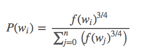
The probability function represent the frequency of the word in the dataset.

Subsampling of Frequent Words

Frequently occurring words often do not provide as much information as a rare word. For example, the word-pair "boat, sea" is likely to occur far more likely than the word "boat, the", yet the former provides the opportunity to encode important contextual information.

This is a typical case: word pairs containing commonly occurring words often do not provide as much information as rare words. Thus, in order to speed up our implementation of Speed-gram, we discard the word [math]\displaystyle{ w_{i} }[/math] from our sample text with probability [math]\displaystyle{ P(w_{i})=1-\sqrt{\frac{t}{f(w_{i}}} }[/math] where [math]\displaystyle{ f(w_{i}) }[/math] is the frequency of word [math]\displaystyle{ w_{i} }[/math] and [math]\displaystyle{ t }[/math] is a chosen threshold, typically around [math]\displaystyle{ 10^{-5} }[/math].

As the probability of encountering a word decreases, the chance of discarding it decreases and approaches 0 as the frequency of the word approaches [math]\displaystyle{ 10^{-5} }[/math]. The figure [math]\displaystyle{ t }[/math] was chosen empirically as it was shown to work well in practice; the chosen threshold aggressively sub-samples words that appear more frequently than [math]\displaystyle{ t }[/math] while preserving the ranking of the frequencies. One thing to note is that the function [math]\displaystyle{ P(w_{i}) }[/math] can have undefined behavior if a word with frequency less than [math]\displaystyle{ t }[/math] occurs; a simple solution is to fix [math]\displaystyle{ P(w_{i}) = 0 }[/math] for any such word.

This procedure provides a significant speedup to our algorithm as there are a lot of frequently occurring words that can be cut, yet they often encode minimally important information. As the results show, both accuracy and training speed increase.

Empirical Results

To evaluate the results of these optimization, Mikolov and Al. used an internal dataset at Google. This dataset contains 1 billions. By removing all workings which occured less than 5 times, dataset size dropped to 692K words. Two type of data analogies where looked at: syntactic and semantic analogies. Syntactic analogies is when two words have the same meaning but describe two different things (e.g. “quick” : “quickly” :: “slow” : “slowly”). Semantic is when two pairs of words have the same vector meaning. For example, “Berlin” : “Germany” and “Paris” : “France” are semantic analogies.

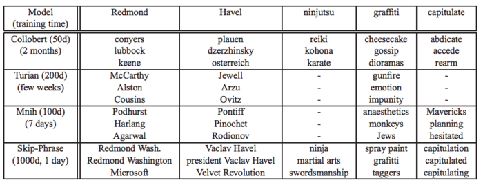
Finally, the model was compared to state of art models from 2013 to evaluate their accuracy. The word2vec project was trained on a dataset of 30 billions words with 1000 dimensions. A sample of its results for less used words compared the models by Collobert, Turian, and Mnih are shown below. We can see the Skip-Phrase is comparatively a lot faster to run and produce every accurate results.

References

[1] McCormick, C. (2017, January 11). Word2Vec Tutorial Part 2 - Negative Sampling. Retrieved from http://www.mccormickml.com

[2] McCormick, C. (2016, April 19). Word2Vec Tutorial - The Skip-Gram Model. Retrieved from http://www.mccormickml.com

[3] Tomas Mikolov, Ilya Sutskever, Kai Chen, Greg Corrado, Jeffrey Dean (2013). Distributed Representations of Words and Phrases and their Compositionality. arXiv:1310.4546. (The paper in question)

[4] Tomas Mikolov, Kai Chen, Greg Corrado, Jeffrey Dean (2013). Efficient Estimation of Word Representations in Vector Space. arXiv:1301.3781 (Earlier paper)