Robust Probabilistic Modeling with Bayesian Data Reweighting
This is a summary based on the paper, Robust Probabilistic Modeling with Bayesian Data Reweighting by Wang, Kucukelbir, and Blei.
Probabilistic models approximate the distribution of data to help with analysis and prediction by relying on a set of assumptions. Data points which deviate from these assumptions can undermine inference and prediction quality. Robust Probabilistic Modeling through Bayesian Data Reweighting helps "robustify" probabilistic models so they can identify and down-weight outlying data points.
Presented By
- Qingxi Huo
- Jiaqi Wang
- Colin Stranc
- Aditya Maheshwari
- Yanmin Yang
- Yuanjing Cai
- Philomene Bobichon
- Zepeng An
Motivation
Imagine a Netflix account belonging to a young child. She has watched many animated kids movies. Netflix accurately recommends other animated kids movies for her. One day her parents forget to switch to their Netflix account and watch a horror movie.
Recommendation models, like Poisson Factorization struggle with this kind of corrupted data: it begins to recommend horror movies to the kid.
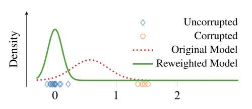
Graphically, the blue diamonds represent kids movies and the green circles are horror movies. The kids movies lay close to each other along some axis. If they were the only observations, the original model would have no troubles identifying a satisfactory distribution. The addition of the horror movies however, pulls the original model so it is centered at [math]\displaystyle{ \approx0.6 }[/math] instead of [math]\displaystyle{ 0 }[/math].
The reweighted model does not have this problem. It chooses to reduce the influence of the horror movies and strongly favours the underlying distribution of the kids movies.
Overview
Reweighted probabilistic modelling works at a high level as follows:
- Define a probabilistic model [math]\displaystyle{ \pi(\beta)\prod_{n=1}^{N}L(y_n|\beta) }[/math]
- Raise each [math]\displaystyle{ L(y_n|\beta) }[/math] to a positive latent weight [math]\displaystyle{ w_n }[/math]. Choose a prior for the weights [math]\displaystyle{ \pi(\boldsymbol{w}) }[/math] where [math]\displaystyle{ \boldsymbol{w} = (w_1,...,w_n) }[/math].
- This gives the RPM (1) with log likelihood (2):
- [math]\displaystyle{ (1) \quad p(\boldsymbol{y}, \boldsymbol{\beta}, \boldsymbol{w}) = \frac{1}{Z}\pi(\boldsymbol{\beta})\pi(\boldsymbol{w})\prod_{n=1}^{N}L(y_n|\boldsymbol{\beta})^{w_n} }[/math]
- [math]\displaystyle{ (2) \quad \log p(\boldsymbol{y}, \boldsymbol{\beta}, \boldsymbol{w}) = \log \pi(\boldsymbol{\beta})+\log \pi(\boldsymbol{w})+\sum_{n=1}^{N}w_n l(y_n|\boldsymbol{\beta}) }[/math]
- A weight close to 0 flattens the likelihood [math]\displaystyle{ l(y_n|\boldsymbol{\beta}) }[/math], but also reduces the overall likelihood. Therefore, only extremely unlikely points will be flattened (down-weighted), and the rest of the likelihoods will be peaked.
- Infer the latent variables [math]\displaystyle{ \beta }[/math] and the weights [math]\displaystyle{ \boldsymbol{w} }[/math], [math]\displaystyle{ p(\boldsymbol{\beta}, \boldsymbol{w}|\boldsymbol{y}) \propto p(\boldsymbol{y}, \boldsymbol{\beta}, \boldsymbol{w}) }[/math]
There are 3 common options for prior on weights [math]\displaystyle{ \boldsymbol{w} }[/math]:
- Bank of Beta priors: (Preferred)
- [math]\displaystyle{ \pi(\boldsymbol{w}) = \prod_{n=1}^{N}\beta(w_n; a, b), ~ where ~ w_n \in (0,1) }[/math]
- Scaled Dirichlet prior
- [math]\displaystyle{ \boldsymbol{w} = N\boldsymbol{v} }[/math]
- [math]\displaystyle{ p_{\boldsymbol{v}}(\boldsymbol{v}) = \text{Dirichlet}(a\boldsymbol{1}) }[/math]
- This ensures sum of the weights equal to N. Analogous to [math]\displaystyle{ \beta }[/math] distribution, small [math]\displaystyle{ a }[/math] allows the model to up- or down-scale weights [math]\displaystyle{ \boldsymbol{w} }[/math] more easily.
- Bank of Gamma Priors
- [math]\displaystyle{ \pi(\boldsymbol{w}) = \prod_{n=1}^{N} Gamma(w_n;a,b) }[/math]
- Not recommended because observations can be arbitrarily up- or down-weighted.
Theory and Intuition
Taking the partial derivative of the density function of RPM and plugging in the Gamma prior, we can estimate [math]\displaystyle{ \boldsymbol{w_n} }[/math] with:
This equation indicates that [math]\displaystyle{ \boldsymbol{w_n} }[/math] shrinks the contribution of observations that are unlikely under the log likelihood since [math]\displaystyle{ \boldsymbol{w_n} }[/math] is an increasing function of the log likelihood of [math]\displaystyle{ y_n }[/math]. Also, it establishes sufficient conditions where a RPM to improve the inference of its latent variable [math]\displaystyle{ \beta }[/math].
The influence function (IF) of [math]\displaystyle{ \bar \beta_w }[/math] shows the amount of improvement, where [math]\displaystyle{ \bar \beta_w }[/math] is the posterior mean of [math]\displaystyle{ \beta }[/math] under weighted model.
We will define the IF function to be:
for z where this limits exists. This IF function roughly describes the asymptotic bias on T(F) cause by a specific observation z that does not come from F. In that case, if there exists an outlier, it will only have small effect, thus the probabilistic model is more robust. It can be proven that if a random value z has likelihood [math]\displaystyle{ l(z|\beta^{\star}) }[/math] that is nearly zero (z is corrupted), then the IF function is also nearly zero. Since the IF function measures how much an additional observation at z affects the statistic T(F). Thus, this corrupted z value will have small effect on the statistic T(F).
Inference and Computation
The likelihood function does not have a closed form solution in all but the simplest of cases. Optimal values for [math]\displaystyle{ \beta }[/math] and [math]\displaystyle{ w }[/math] are therefore solved for using various optimization methods. The paper suggests using automated inference in the probabilistic programming system, STAN.
The RPM's can be measured based on how well they detect and mitigate different forms of mismatch by comparing the predictive accuracy on held out data for the original, localized, and re-weighted models.
Exmples
Ignoring Outliers
Our observations are a routers wait times for packets. These wait times follow a [math]\displaystyle{ POIS\left( 5 \right) }[/math] distribution. The network can fail, which is modelled by wait times following a [math]\displaystyle{ POIS\left( 50 \right) }[/math] distribution instead.
A Gamma prior is chosen for the rate. The network is set to fail [math]\displaystyle{ 25 }[/math]% of the time.
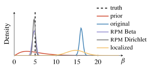
Note that the reweighted models accurately detected the rate whereas the other models did not. Notice also that the reweighted models had a much smaller spread than most other models.
This shows that BDR can handle data from an unrelated distribution.
Handling Missing Latent Groups
We are attempting to predict the number of people who are colour blind, but we do not know whether the individual is male or female. Men are inherently more likely to be colour blind than females, so without gender information a standard logistic regression would misrepresent both groups. Bayesian Reweighting identifies the different distributions and only reports on the dominant group.
For the example we simulate data points from different Bernoulli distributions for men and women. We examine the results with varying degrees of the population being female.
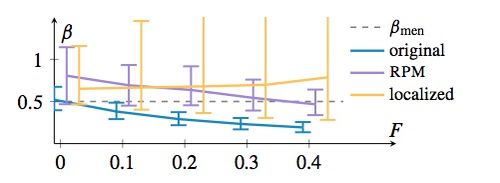
Note here that the RPM model always contains the true mean in its [math]\displaystyle{ 95 }[/math]% credible interval. The localized model also contains the mean, however it contains much less certainty in it's predictions.
We can see that the RPM model successfully ignored the observations which came from the minority distribution, without any information on its existence.
Lung Cancer Risk Study
We have three models of lung cancer risk dependency on tobacco usage and obesity and we distinguish the true model and the assumed model by some form of covariance misspecification in each model.

Note that RPM yields better estimates of [math]\displaystyle{ \beta_1 }[/math] in the first two models but gives a similar result to the original model in the third model where the obesity is ignored in the misspecified model.
This shows that RPM leverages datapoints are useful for estimating [math]\displaystyle{ \beta_1 }[/math] and RPMs can only use available information.
Cluster Selection in a Mixture Model
This example shows how RPMs handle skewed data. We apply RPM on a Dirichlet process mixture model (DPMM). DPMM is a versatile model for density estimation and clustering, and a reweighted DPMM reliably recovers the correct number of components in a mixture of skewnormals dataset.
We simulate three clusters from two-dimensional skewnormal distribution (N = 2000).
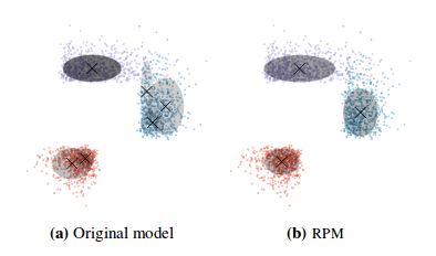
When fitting an approximate DPMM to the dataset, it incorrectly finds six clusters. In contrast, the RPM identifies the correct three clusters. The result shows that RPM down-weights the datapoints that do not match the Gaussianity assumption of the model.
Real Data (MovieLens 1M)
To test the model on real data, we use the MovieLens data set. It contains [math]\displaystyle{ 6000 }[/math] users ratings of a total of [math]\displaystyle{ 4000 }[/math] movies. We train a RPM model on the clean data, then add varying degrees of random corruption and see how an RPM model handles that data.
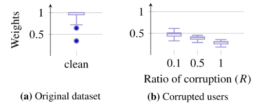
Notice the clean data provides almost entirely weights near [math]\displaystyle{ 1 }[/math]. Once corrupt data is created we see view only the weights for those corrupt data points. Notice that they tend to get lower and lower the more corrupted their ratings are.