Summary - A Neural Representation of Sketch Drawings
This paper discusses sketch-rnn, a sequence-to-sequence Variational Autoencoder for generating new vector images images from a given set of hand drawn vector images. The focus on vector images is based on the reasoning that they are a much better representation of how human beings create drawings than the traditional pixel approach. Vector images created by sketch-rnn can be conditioned on a given image, or generated unconditionally by sampling from a learned distribution. Creating new sketches in this way allows neural networks like sketch-rnn opens the possibility of many applications: to be used as a way to teach children to draw, or extend the capacity of an artist by generating many possible next steps for a given sketch.
Related Work
Most work in the area of image generating neural networks has dealt with pixel base images rather than vector based images. There has been some work with a similar aim to this paper, attempting to generate handwriting using Recurrent Neural Networks (Graves, 2013), and other investigations into creating vectorized Kanji characters (Ha, 2015; Zhang et al., 2016). Use of sequence-to-sequence architecture with a Variational Autoencoder had been previously applied to modelling natural language (Bowman et al., 2015), but sketch-rnn takes a new step by using the same combination and applying it to vector images.
Background: The Building Blocks of sketch-rnn
Variational Autoencoders (VAEs)
A variational autoencoder (VAE) is a classical autoencoder and is a neural network consisting of an encoder, a decoder and a loss function. They can be used for image generation and reinforcement learning as they let us design generative models of data and fit them to large data-sets.
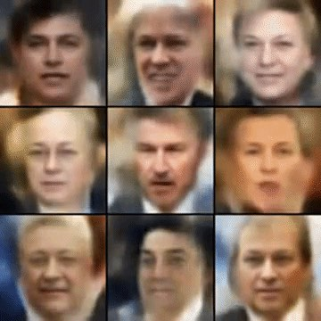
Figure 1: Examples of generated images of faces
Simply, the VAE first layer is the encoder which take the input and convert it into a latent vector by reducing the mean squared error of the input and output, like a standard autoencoder. Then to make VAE a generative model, the generate latent vectors should roughly follow a Gaussian distribution as shown in Fig.1. This allows the user to generate an output similar to the database the VAE was trained on by inputting a latent vector straight to the decoder.
Figure 2: Structure of a VAE
Given data in the form of [math]\displaystyle{ X }[/math]’s which are encoded to [math]\displaystyle{ z }[/math]’s, our goal is to maximize the expectation of generating a real data point [math]\displaystyle{ X }[/math] given an encoding [math]\displaystyle{ z }[/math] and parameters :
P(X|z, )P(z)dz = EzP(z)[P(X|z,)]
Where is an optimizing parameter so that [math]\displaystyle{ z }[/math] can be sampled from [math]\displaystyle{ P(z) }[/math] with high probability that f(z;θ) or P(X|z, ) is most likely be one of the [math]\displaystyle{ X }[/math]’s in our dataset. However, a given [math]\displaystyle{ z }[/math] from [math]\displaystyle{ P(z) }[/math] is unlikely to produce a reasonable [math]\displaystyle{ X }[/math]. The challenge is to sample from the posterior distribution [math]\displaystyle{ P(z|X) }[/math] because it allows [math]\displaystyle{ z }[/math] to be conditioned on real data, making a latent vector sampled from it more likely to produce realistic results. Unfortunately, we can’t sample from the posterior. To fix this, we sample instead from a distribution approximating [math]\displaystyle{ P(z|X) }[/math] that is easily sampled from: Q(z|X)N(, ) Now there are two requirements to take into account: [math]\displaystyle{ Q(z|X) }[/math] must approximate [math]\displaystyle{ P(z|X) }[/math] reasonably well, and P(X|)must be maximized. Then our objective has the form: $$ \log(P(X|\theta)) - K_{DL}[Q(z|X,\theta)||P(z|X,\theta)] = E_{z\simQ(z|X,\theta)}[\log(P(X|z,\theta)] - K_{DL}(Q(z|X,\theta)||P(z|\theta)) $$ It is important to note that using [math]\displaystyle{ Q(z|X)\simN(\mu, \Sigma) }[/math] allows the encoder to output the parameters necessary to create [math]\displaystyle{ z }[/math] with the desired distribution by defining [math]\displaystyle{ z }[/math] as [math]\displaystyle{ z }[/math] =+1/2*where is sampled from [math]\displaystyle{ N(0, 1) }[/math]. This also allows the VAE to be trained using back propagation since the random part of [math]\displaystyle{ z }[/math] ([math]\displaystyle{ \epsilon }[/math]) is sampled separately from the flow of gradients in the encoder/decoder.
Recurrent Neural Networks (RNNs)
RNNs are closely related to Feed Forward Neural Networks, but have a few properties that make them suited to modeling sequential data. Consider a sequence of vectors [math]\displaystyle{ x_1, x_2, x_3...x_n }[/math] representing the individual strokes of a drawing similar to the data used by sketch-rnn. It is important to take into account previous strokes if we are to learn patterns in drawings. An RNN satisfies this requirement by retaining a “memory” of the hidden states of previous strokes and uses it to inform output. RNNs are highly effective in modelling many types of sequential data such as natural language and drawings.
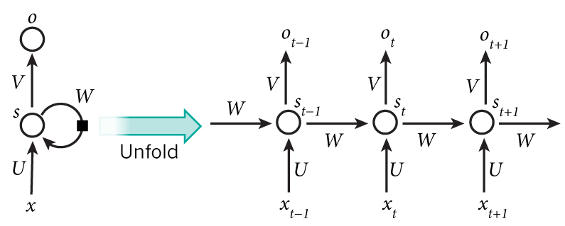
Figure 3: An RNN and it’s unfolded counterpart
Figure 3 shows the basic structure of an RNN on the left. On the right is it’s “unrolled” equivalent, very similar to an FFNN, but with an extra input at the hidden layer. For example, the output of the hidden layer after the input of [math]\displaystyle{ x_t }[/math] is [math]\displaystyle{ s_t=f(Ux_t+Ws_{t-1}) }[/math]. Here, [math]\displaystyle{ f }[/math] is the activation function applied to every element of the vector [math]\displaystyle{ Ux_t+Ws_{t-1} }[/math], [math]\displaystyle{ x_t }[/math] is the input, [math]\displaystyle{ U }[/math] and [math]\displaystyle{ W }[/math] are the matrices of weights and [math]\displaystyle{ s_{t-1} }[/math] is the hidden state of the previous data [math]\displaystyle{ x_{t-1} }[/math].
RNNs can be trained using backpropagation, and since all weights in [math]\displaystyle{ U }[/math], [math]\displaystyle{ W }[/math] and [math]\displaystyle{ V }[/math] are shared by each unrolled layer, there are much fewer parameters to train than a FFNN with the same number of layers.
QuickDraw Data Set
The sketch-rnn model was trained and tested using the QuickDraw data set. This data set consists of drawings obtained from the Quick, Draw! game where players are asked to draw a picture of a given object. Drawn objects are stored in a format that captures the pen stroke actions. Each action is given as a vector of 5 items, (x, y, p1, p2, p3). (x,y)gives the offset of the pen from the previous point. (p1, p2, p3)are a binary one-hot of possible states for the pen. Respectively, they indicate if the pen is touching the paper, that the pen is about to be lifted from the paper and no line will be drawn next, and that the drawing is finished.
Loss Functions
The training procedure for sketch-rnn uses a combination of two loss functions, Reconstruction loss (LR) and Kullback-Liebler Divergence (LKL). The former optimizes the log-likelihood of the generated probability distribution to explain the training data, and the latter optimizes the difference between the distribution of the latent vector and an independently identically distributed standard normal vector. The objective function is a weighted combination of these two loss functions, Loss = Lr+KLLKL. KL is a hyperparameter that controls the behaviour of the model. For KL0, the model acts as a pure encoder. It decreases the reconstruction loss of the model, but sacrifices the ability to enforce a prior over the latent space. For training, the loss function was further modified by adding a weight growth to the Kullback-Liebler part of the loss function. Loss=LR+KL(1-(1-min)Rstep) max{LKL,KLmin} for some min,R < 1. The contribution of the Kullback-Liebler term to the loss function therefore starts small (if R close to 1) and approaches KLLKL with each step. This was added to allow the optimizer to first focus on reconstruction, which is optimized by the LRloss, and later optimize for the LKL term. However, a minimum value of the LKLterm was enforced by taking max{LKL,KLmin} for some floor KLmin, as it was found that decreasing the LKL loss did not lead to further improvements in the decoder beyond a certain value of LKL. The minimum value for KLmin therefore encourages the optimizer to focus on minimizing the LRterm and improving reconstruction loss once the LKL term is low enough. For the majority of the experiments described in this paper, the model was configured with R=0.99999, KLmin=0.2,KL =1,min=0
Methodology and Experiment
Encoder
The purpose of the encoder is to ingest an image sketch [math]\displaystyle{ x }[/math] and produce vectors [math]\displaystyle{ \mu }[/math] and [math]\displaystyle{ \sigma }[/math] whose [math]\displaystyle{ N_z }[/math] entries parameterize the [math]\displaystyle{ N_z }[/math] univariate Gaussian distributions from which the [math]\displaystyle{ N_z }[/math] entries of the latent vector [math]\displaystyle{ z }[/math] are generated. The latent vector [math]\displaystyle{ z }[/math] is the [math]\displaystyle{ N_z }[/math] dimensional embedding of the image sketch [math]\displaystyle{ x }[/math] like the latent vector of a standard variational autoencoder, or similar to a standard autoencoder but not a deterministic function of [math]\displaystyle{ x }[/math]
That is, they parameterize [math]\displaystyle{ Q(z|x) }[/math] as described in the background (which is, in this model, multivariate gaussian but with covariances 0, and the entries of vector along the diagonal)
Intuitively, the mean vector [math]\displaystyle{ \mu }[/math] estimates the location of the images in latent space. If one were to consider all latent vectors corresponding to a single class in the training data, ideally they would be close together.
The encoder takes the form of a bidirectional RNN consisting of two standard RNNs which are run along a sketch sequence in temporal and reverse temporal order, respectively, whose output vectors are concatenated to form a vector [math]\displaystyle{ h }[/math]. The vector [math]\displaystyle{ h }[/math] is then projected to [math]\displaystyle{ \mu }[/math] and [math]\displaystyle{ \sigma }[/math] via the following transformations:
[math]\displaystyle{ \mu =W_\mu h + b\mu }[/math] [math]\displaystyle{ \sigma=exp(\frac{W_\sigma h + b_\sigma}{2}) }[/math]
Where the exponential operation is required to make positive and hence a valid variance. The latent vector is then generated as [math]\displaystyle{ z = \mu + \sigma \odot \mathcal{N}(0, 1) }[/math], where [math]\displaystyle{ \odot }[/math] is the entrywise product of vectors and the latter term is an [math]\displaystyle{ N_z }[/math]-length vector each of whose entries is generated from [math]\displaystyle{ N(0, 1) }[/math] . This is important because when the encoder is trained along with the decoder in end-to-end backpropagation, [math]\displaystyle{ z = \mu + \sigma \odot \mathcal{N}(0, 1) }[/math] can be treated as an affine transformation of some constant, so the derivative of the loss can be taken with respect to both of these parameters.
Decoder
The purpose of the decoder is to parameterize the distribution [math]\displaystyle{ P(x|z) }[/math]. It takes a latent vector [math]\displaystyle{ z }[/math] and generates a sketch. It is modelled by another RNN, which at each timestep [math]\displaystyle{ i }[/math] takes the point outputted by the previous step, [math]\displaystyle{ S_{i-1} }[/math] (where [math]\displaystyle{ S_0= (0, 0, 1, 0, 0)) }[/math] and the latent vector [math]\displaystyle{ z }[/math], in addition to passing the hidden state [math]\displaystyle{ h_i }[/math] between steps. The output of node [math]\displaystyle{ i }[/math] is the parameters of a Gaussian mixture model for the differents coordinates of pointi from the point [math]\displaystyle{ i-1 }[/math] of the sketch, and the probabilities [math]\displaystyle{ (q_1, q_2, q_3) }[/math]. The Gaussian mixture model is a weighted sum of Mbivariate normal distributions, where [math]\displaystyle{ M }[/math] is a hyperparameter and hence is written as
[math]\displaystyle{ p(\Delta x, \Delta y) = \sum_{j=1}^M\Pi_j \mathcal{N}(\Delta x, \Delta y | \mu_{x, j}, \mu_{y, j}, \sigma_{x,j}, \sigma_{y, j}, \rho{xy, j}) }[/math]
Where [math]\displaystyle{ \sum_{j=1}^M Pi_j=1 }[/math]. Thus the a given node of the RNN must return [math]\displaystyle{ 6M+3 }[/math] parameters in total, where the first [math]\displaystyle{ 6M }[/math] parameterize the mixture model and the remaining 3 are [math]\displaystyle{ (\hat{q_1}, \hat{q_2}, \hat{q_3}) }[/math]. This means each RNN must output
[math]\displaystyle{ y_i = [(\hat{\Pi},\mu_x,\mu_y, \hat{\sigma_x},\hat{\sigma_y},\hat{\rho})_1, ..., (\hat{\Pi},\mu_x,\mu_y, \hat{\sigma_x},\hat{\sigma_y},\hat{\rho})_M, (\hat{q_1}, \hat{q_2}, \hat{q_3})] }[/math]
which is computed by
[math]\displaystyle{ y_i = W_y h_i + b_y }[/math]
This produces a [math]\displaystyle{ 6M+1 }[/math] -length vector [math]\displaystyle{ yi }[/math]. In order to make the parameters valid, the following conditions must be met:
[math]\displaystyle{ \sum_{j=1}^M \Pi_j = 1 }[/math]
[math]\displaystyle{ q_1 + q_2 + q_3 = 1 }[/math]
[math]\displaystyle{ \sigma_{x, j}, \sigma_{y, j}\gt 0 }[/math]
[math]\displaystyle{ -1 \lt \rho_{xy, j} \lt 1 }[/math].
To meet these, we set
[math]\displaystyle{ \Pi_i = \frac{e^{\hat{\Pi_i}}}{\sum_{k=1}^M e^{\hat{\Pi_i}}} }[/math]
[math]\displaystyle{ q_i = \frac{e^{\hat{q_i}}}{\sum_{k=1}^M e^{\hat{q_i}}} }[/math]
[math]\displaystyle{ \sigma_{x, j} = e^{\hat{\sigma_{x_j}}} }[/math]
[math]\displaystyle{ \sigma_{y, j} = e^{\hat{\sigma_{y_j}}} }[/math]
[math]\displaystyle{ \rho_{xy, j} = e^{\hat{\tanh_{\rho_{xy, j}}}} }[/math]
We then draw [math]\displaystyle{ S_i }[/math] from the resulting posterior distribution, and [math]\displaystyle{ x }[/math] is computed using all such points [math]\displaystyle{ Si }[/math].
Unconditional Generation
As an interesting aside, the decoder can be trained without the encoder to generate sketches with no prior (latent vector) [math]\displaystyle{ z }[/math]. The decoder is simply adjusted not to concatenate a latent vector to the input of each time step, then trained using only the reconstruction loss (during which this term will become somewhat of a misnomer, as there is no input to be reconstructed in this process).
Experiments
To analyse sketch-rnn, we perform experiments for both conditional and unconditional image generation. We train several models and then analyse the uses of these trained models. We use Long Short-Term Memory (LSTM) (Hochreiter & Schmidhuber, 1997) as the encoder RNN and we use HyperLSTM for the decoder RNN.
Using the QuickDraw dataset, in particular, the classes (cat, pig, face, firetruck, garden, owl, mosquito and yoga class) we train various models individually on these classes and then 2 models were trained on multiple classes (cat, pig) and (crab, face, pig, rabbit). In training, various [math]\displaystyle{ w_{KL} }[/math] were used and the breakdown of the losses [math]\displaystyle{ L_{R} }[/math] and [math]\displaystyle{ L_{KL} }[/math] were recorded.The results of the experiments are shown below:
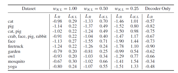
From the table, we see that as we relax (i.e. decrease) [math]\displaystyle{ w_{KL} }[/math](the weight for the KL loss term), [math]\displaystyle{ R_L }[/math] (the reconstruction loss) decreases and [math]\displaystyle{ L_{KL} }[/math] (KL loss) increases. This result can be seen visually in the training section above.
After training a sketch-rnn models we can use them in 4 ways:
- Conditional Reconstruction
- Latent Space Interpolation
- Sketch Drawing Analogies
- Predicting Different Endings of Incomplete Sketches
Conditional Reconstruction
In this application, we can use a sketch-rnn model to reconstruct an image based on a given input.For example, using a model trained only on the cat class based on a given input, we can reconstruct cat sketch. This is shown in the figure below.

In the above image, we view results, based on levels of temperature [math]\displaystyle{ \tau }[/math] from (0.01, to 1). This is represented by a blue to pink color scheme.
The first thing we notice is that for lower levels of [math]\displaystyle{ \tau }[/math], the model produces results that closely mirror the input.
The second thing we notice is the image reconstruction of images that do not have the typical features of a cat (i.e. noisy input). When the input is a cat with 3 eyes, the reconstructed cat only has 2 eyes and when the input is a toothbrush, the model keeps the shape of the toothbrush but gives it cat features. In the above figure, we also show similar results for a pig only model.
Latent Space Interpolation
In this application, we use a model trained on 2 classes (in this case, cat and pig and view how one class morphs into the other class. The color scheme blue to pink represent stages as the model morphs the input. In the below image, we view results of the reconstructions on the interpolations from cat to pig, using models trained with various levels of [math]\displaystyle{ w_{KL} }[/math].
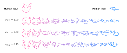
Notice that with [math]\displaystyle{ w_{KL}=0.25 }[/math] the reconstruction is poor and is a replica of the original input, whereas with [math]\displaystyle{ w_{KL}=1 }[/math] , the reconstruction is good and we have a distinct image of a pig at the end.
Recall, that as [math]\displaystyle{ w_{KL} }[/math] decreases, [math]\displaystyle{ L_R }[/math] decreases and [math]\displaystyle{ L_{KL} }[/math] increases. With a lower [math]\displaystyle{ L_{KL} }[/math] we see that the model will generate coherent images regardless of how noisy the input is. This is because, with lower [math]\displaystyle{ L_{KL} }[/math], the encoded latent vectors contain conceptual features of the input sketch while with higher [math]\displaystyle{ L_{KL} }[/math], the encoded latent vectors only contain information on the specific line segments. This suggests that when training a model, we must always investigate the trade-off between the two loss terms as this will affect the quality of the reproduced sketch.
Sketch Drawing Analogies
In this application, using an input sketch, we augment features of a sketch. This means that we take an input sketch of a class and then add features from another class to that sketch (i.e. we investigate the features in the model’s latent space).
As mentioned above, the latent vectors contain information on the features of the input sketch. Models with Low [math]\displaystyle{ L_{KL} }[/math], contain conceptual features of a sketch and hence we can use the latent vectors of these models to augment sketches. This can be seen below.
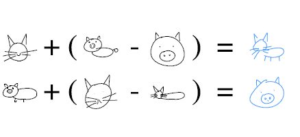
In the above image, in the first row, we first subtract the latent vector of an encoded pig head from the latent vector of a full pig to produce a sketch that would represent a “body”. We then use this “body and attach it to a cat head to produce a full cat.In the second row, we do the opposite We take the latent vector of encoded full cat from the latent vector of cat head to represent the action “subtract body”. We then add this to a full pig sketch to produce a sketch of a pig head.
Predicting Different Endings of Incomplete Sketches
With this application, we can give a decoder only model trained on a single class an incomplete sketch as in input (i.e. a series of lines) and then predict various possible endings for that given input. This is shown below with [math]\displaystyle{ \tau=0.8 }[/math].
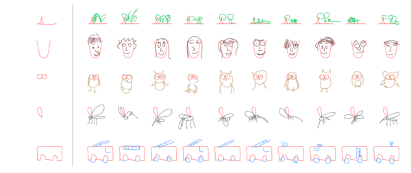
Using this type of model, we first encode the sketch into a complete hidden state, h and then generate a sketch that is conditioned on the points from h.
Application and Future Work
The model sketch-rnn can help assist artists through the creative process. Whether it is by drawing many unique images for a design, creating uncommon abstract art, with a high wkl and low temperature the model will transform a poorly sketched drawing into a more coherent version of itself.
The paper can be continued by combining the sketch-rnn model with unsupervised, cross-domain pixel generation models. The idea would be to take a photograph of an image and decompose it into a hand drawn image. The challenge would be to limit the lines in the sketch while still producing a coherent image.
Criticism
The sketch-rnn model is a RNN-VAE, which uses three RNNs in the model. RNNs suffer from the vanishing gradient problem. This problem stems not from the gradient becoming small but from the long-term dependencies becoming small while the short-term dependencies expand. Impling that RNN models can learn in the short-term but forget long-term information. Sketch-rnn attempts to counter this by using LSTM models to encode and decode the images. LSTM is a proposed solution to the vanishing gradient problem by Hochreiter & Schmidhuber (1997). LSTM adapts the RNN model by instead of computing St by St-1 directly it added the gradient 𝚫St to St-1. It then uses this new value to compute St. This change prevents the long-term gradients to fully disappear. But after enough iterations (1000s or 10000s) the gradients will lose information.
The model also has problems scaling to larger images. For the current applications of sketch-rnn the images drawn only require 200-300 timesteps. As mentioned in the paper’s supplementary material the model has difficulty training on more then 300 data points. This could implies that the model is difficult to scale to larger problems or drawings. If one was trying to implement a much more detailed drawing this model would have difficulty dealing with the extra data points.
Another limitation is the scalability of the model to multiple different classes. As per mention within the supplementary material, the model tends to start combining features from different class when ask to construct a sketch action when the model is given 4 or more concatenated class. This presented some limitations since multiple model is required in order to have a model to generate sketches for multiple classes. Although there has been effort by GPU manufacturer such Nvidia to optimize the training algorithm, RNN is still remains a computationally expensive model to train. These limitations will hinder the practicality of the model.
In terms of presentation, Ha and Eck have done a great job in explaining the details of the model within the paper. The paper was extremely approachable even to someone with minimal background. Their decision to leave some of the details to supplementary material also allowed the reader to grasp the general outline without overwhelming the reader. However, the author’s decision to only included successful result in the main paper, and left the limitation of the model within the supplementary material harms the overall credibility of the paper. There is also no mention of any inaccuracy or bad drawing generated by the model within the paper, which seems odd given that this is a new methodology. This gives the impression that only the selected model within the paper perform well.
References
Alex Graves. Generating sequences with recurrent neural networks. arXiv:1308.0850, 2013.
David Ha. Recurrent Net Dreams Up Fake Chinese Characters in Vector Format with TensorFlow, 2015.
Ha, D., & Eck, D. A Neural Representation of Sketch Drawings. https://iclr.cc/Conferences/2018/Schedule?showEvent=293. (2018)
Doersch, Carl. "Tutorial on variational autoencoders." arXiv preprint arXiv:1606.05908 (2016).
Kurita, Keita. “An Intuitive Explanation of Variational Autoencoders (VAEs Part 1).” Machine Learning Explained, 2 Mar. 2018, https://mlexplained.com/2017/12/28/an-intuitive-explanation-of-variational-autoencoders-vaes-part-1/.
Kurita, Keita. “An Introduction to the Math of Variational Autoencoders (VAEs Part 2).” Machine Learning Explained, 2 Mar. 2018, https://mlexplained.com/2017/12/28/an-introduction-to-the-math-of-variational-autoencoders-vaes-part-2/.
Samuel R. Bowman, Luke Vilnis, Oriol Vinyals, Andrew M. Dai, Rafal Józefowicz, and Samy Bengio. Generating Sentences from a Continuous Space. CoRR, abs/1511.06349, 2015. URL http://arxiv.org/abs/1511.06349.
Xu-Yao Zhang, Fei Yin, Yan-Ming Zhang, Cheng-Lin Liu, and Yoshua Bengio. Drawing and Recognizing Chinese Characters with Recurrent Neural Network. CoRR, abs/1606.06539, 2016. URL http://arxiv.org/abs/1606.06539.
Recurrent Neural Networks Tutorial, Part 1 – Introduction To Rnns , Denny Britz - http://www.wildml.com/2015/09/recurrent-neural-networks-tutorial-part-1-introduction-to-rnns/
Jozefowicz, Rafal, Wojciech Zaremba, and Ilya Sutskever. "An empirical exploration of recurrent network architectures." International Conference on Machine Learning. 2015.
Jeremy Appleyard “Optimizing Recurrent Neural Networks in CuDNN5”, https://devblogs.nvidia.com/optimizing-recurrent-neural-networks-cudnn-5/ , Apr. 6 2016
