Memory-Based Parameter Adaptation
This is a summary based on the paper, Memory-based Parameter Adaptation by Sprechmann et al.[1].
The paper generalizes some approaches in language modelling that seek to overcome some of the shortcomings of neural networks including the phenomenon of catastrophic forgetting using memory-based adaptation. Catastrophic forgetting occurs when neural networks perform poorly on old tasks after they have been trained to perform well on a new task. The paper also presents experimental results where the model in question is applied to continual and incremental learning tasks.
Presented by
- J.Walton
- J.Schneider
- Z.Abbas
- A.Na
Introduction
Model-based parameter adaptation (MbPA) is based on the theory of complementary learning systems which states that intelligent agents must possess two learning systems, one that allows the gradual acquisition of knowledge and another that allows rapid learning of the specifics of individual experiences[2]. Similarly, MbPA consists of two components: a parametric component and a non-parametric component. The parametric component is the standard neural network which learns slowly (low learning rates) but generalizes well. The non-parametric component, on the other hand, is a neural network augmented with an episodic memory that allows storing of previous experiences and local adaptation of the weights of the parametric component. The parametric and non-parametric components therefore serve different purposes during the training and testing phases.
Model Architecture

Training Phase
The model consists of three components: an embedding network [math]\displaystyle{ f_{\gamma} }[/math], a memory [math]\displaystyle{ M }[/math] and an output network [math]\displaystyle{ g_{\theta} }[/math]. The embedding network and the output network can be thought of as the standard feedforward neural networks for our purposes, with parameters (weights) [math]\displaystyle{ \gamma }[/math] and [math]\displaystyle{ \theta }[/math], respectively. The memory, denoted by [math]\displaystyle{ M }[/math], stores “experiences” in the form of key and value pairs [math]\displaystyle{ \{(h_{i},v_{i})\} }[/math] where the keys [math]\displaystyle{ h_{i} }[/math] are the outputs of the embedding network [math]\displaystyle{ f_{\gamma}(x_{i}) }[/math] and the values [math]\displaystyle{ v_{i} }[/math], in the context of classification, are simply the true class labels [math]\displaystyle{ y_{i} }[/math]. Thus, for a given input [math]\displaystyle{ x_{j} }[/math]
[math]\displaystyle{ f_{\gamma}(x_{j}) \rightarrow h_{j}, }[/math]
[math]\displaystyle{ y_{j} \rightarrow v_{j}. }[/math]
Note that the memory has a fixed size; thus when it is full, the oldest data is discarded first.
During training, the authors sample of a set of [math]\displaystyle{ b }[/math] training examples randomly (ie. mini-batch size [math]\displaystyle{ b }[/math]), say [math]\displaystyle{ \{(x_{b},y_{b})\}_{b} }[/math], from the training data that they input into the embedding network [math]\displaystyle{ f_{\gamma} }[/math], followed by the output network [math]\displaystyle{ g_{\theta} }[/math]. The parameters of the embedding and output networks are updated by maximizing the likelihood function (equivalently, minimizing the loss function) of the target values
[math]\displaystyle{ p(y|x,\gamma,\theta)=g_{\theta}(f_{\gamma}(x)). }[/math]
The last layer of the output network [math]\displaystyle{ g_{\theta} }[/math] is a softmax layer, such that the output can be interpreted as a probability distribution. This process is also known as backpropagation with mini-batch gradient descent. Finally, the embedded samples [math]\displaystyle{ \{(f_{\gamma}(x_{b}),y_{b})\}_{b} }[/math] are stored into the memory. No local adaptation takes place during this phase.
Testing Phase
During the testing phase, the model will temporarily adapt the weights of the output network [math]\displaystyle{ g_{\theta} }[/math] based on the input [math]\displaystyle{ x }[/math] and the contents of the memory, [math]\displaystyle{ M }[/math], according to
[math]\displaystyle{ \theta^x = \theta + \Delta_M. }[/math]
First, [math]\displaystyle{ x }[/math] is inputted into the embedding network, [math]\displaystyle{ q = f_{\gamma}(x) }[/math]. Based on query [math]\displaystyle{ q }[/math], a K-nearest neighbours search is conducted. The contextual, $C$, is the result of this search.
[math]\displaystyle{ C = \{(h_k, v_k, w_k^{(x)})\}^K_{k=1} }[/math]
Each of the neighbours has a weighting [math]\displaystyle{ w_k^{(x)} }[/math] attached to it, based on how close it is to query [math]\displaystyle{ q }[/math]. This calculation is based on the kernel function,
[math]\displaystyle{ kern(h,q) = \frac{1}{\epsilon + ||h-q||^2_2}. }[/math]
The temporary updates during adaptation are based on maximizing the weighted average of the log likelihood over the neighbours in C, also known as the maximum a posteriori over the contextual, [math]\displaystyle{ C }[/math],
[math]\displaystyle{ \max_{\theta^x} \log p(\theta^x | \theta) + \sum^K_{k=1}w_k^{(x)} \log p(v^{(x)}_k | h_k^{(x)}, \theta^x,x). }[/math]
Note that the first term here acts as regularization that prevents over-fitting. Unfortunately, equation 1 does not have a closed form solution. However, it can be maximized using gradient descent in a fixed number of steps. Each of these steps is calculated via [math]\displaystyle{ \Delta M }[/math],
[math]\displaystyle{ \Delta_M (x, \theta) = - \alpha_M \nabla_\theta \sum^K_{k=1} w_k^{(x)} \log p(v^{(x)}_k | h_k^{(x)}, \theta^x,x)\bigg |_\theta - \beta(\theta - \theta^x), }[/math]
where [math]\displaystyle{ \beta }[/math] is a hyper-parameter of gradient descent. After a series of gradient descent steps, the weights of the final output network [math]\displaystyle{ g_{\theta} }[/math] are temporarily adapted and a prediction is made, [math]\displaystyle{ \hat y }[/math].

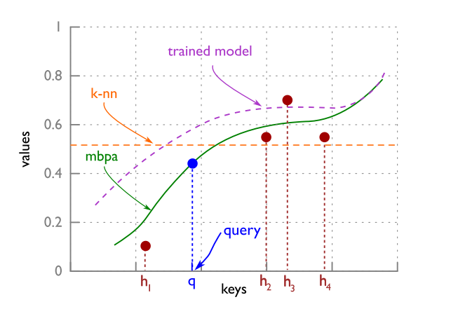
As can be seen in figure 2, the final prediction [math]\displaystyle{ \hat y }[/math] is similar to a weighted average of the values of the K-nearest neighbours.
Examples
Continual Learning
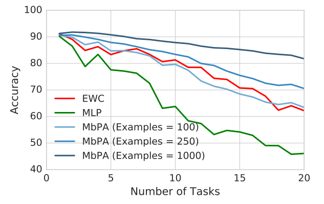
Continual learning is the process of learning multiple tasks in a sequence without revisiting a task. The authors consider a permuted MNIST setup, similar to [3], where each task was given by a different permutation of the pixels. The authors sequentially trained the MbPA on 20 different permutations and tested on previously trained tasks.
The model was trained on 10 000 examples per task, using a 2 layer multi-layer perceptron (MLP) with an ADAM optimizer. The elastic weight consolidation (EWC) method and regular gradient descent were used to estimate the parameters. A grid search was used to determine the EWC penalty cost and the local MbPA learning rate was set as [math]\displaystyle{ \beta\in(0.0,0.1) }[/math] and number of steps (n) was [math]\displaystyle{ n\in[1,20] }[/math].

The authors used the pixels as the embedding, i.e. [math]\displaystyle{ f_{\gamma} }[/math] is the identity function, and looked at regions where episodic memory was small. The authors found that through MbPA only a few gradient steps on carefully selected data from memory is enough to recover performance. They found that MbPA outperformed MLP and worked better than EWC in most cases and found that the performance of MbPA grew with the number of examples stored. They note that the memory requirements were lower than EWC. The lower memory requirements are attributed to the fact that EWC stores all task identifiers, whereas MbPA only stores a few examples. The figure above also shows the results of MbPA combined with other methods. It is noted that MbPA combined with EWC gives the best results.
Incremental Learning
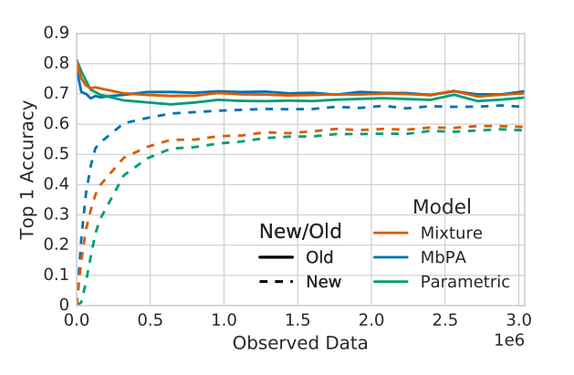
Incremental learning has two steps. First, the model is trained on a subset of the classes found in the training data. The second step is to give it the entire training set and see how long it takes for the model to perform well on the entire set. The purpose of this is to see how quickly the model learns information about new classes and how likely it is to lose information about the old ones. The authors used the ImageNet dataset from [4], and the initial training set contained 500 out of the 1000 classes.
For the first step, they used three models. A parametric model, MbPA, and a mixture model. The parametric model they used was Resnet V1 from [5]. It was used both as the parametric model in MbPA and as a separate model for testing. The non-parametric model used was the memory as described earlier. The memory was created by taking the keys from the second last layer of the parametric model. The mixture model was a convex combination of the outputs of the parametric and non-parametric model as shown below:
[math]\displaystyle{ p(y|q) = \lambda p_{param}(y|q) + (1-\lambda)p_{mem}(y|q). }[/math]
[math]\displaystyle{ \lambda }[/math] was tuned as a hyperparameter. Finally, MbPA was used as the fourth model with the Resnet V1 parametric model, and the non-parametric model being identical to the one described above. They were evaluated using their “Top 1” accuracy. That is to say that the class with the highest output value was taken to be the model’s prediction for a given data point in the test set.

There was also a test on how well the models perform on unbalanced datasets. In addition to the previous three, they included a non-parametric model which was just the memory running without the rest of the network. Since most real-world datasets have different amounts of data in each class, a model that could use unbalanced datasets without becoming biased would have more information available to it for training. The testing here was done similarly to the other incremental learning experiment. The models were trained on 500 of the 1000 classes until they performed well. They were then given a dataset containing all of the data from the first 500 classes and only 10% of the data from the other 500 classes. Accuracy was evaluated both using Top 1 and AUC (area under the curve) accuracy. It was found that after 0.1 epochs, MbPA and the non-parametric model performed similarly and much better than the other two by both accuracy metrics. After 1 or 3 epochs, the non-parametric model begins to perform worse than the others and MbPA continues to perform better.
Conclusion
The MbPA model can successfully overcome several shortcomings associated with neural networks through its non-parametric, episodic memory. In fact, many other works in the context of classification and language modelling have successfully used variants of this architecture, where traditional neural network systems are augmented with memories. Likewise, the experiments in incremental and continual learning presented in this paper use a memory architecture similar to the Differential Neural Dictionary (DND) used in Neural Episodic Control (NEC) found in [6], though the gradients from the memory in the MbPA model are not used during training. In conclusion, MbPA presents a natural way to improve the performance of standard deep networks.
References
- [1]Sprechmann. Pablo, Jayakumar. Siddhant, Rae. Jack, Pritzel. Alexander,Badia. Adria, Uria. Benigno, Vinyals. Oriol, Hassabis. Demis, Pascanu.Razvan, and Blundell. Charles. Memory-based parameter adaptation.ICLR, 2018.
- [2]Kumaran. Dhushan, Hassabis. Demis, and McClelland. James. What learning systems do intelligent agents need? Trends in Cognitive Sciences,2016.
- [3]Goodfellow. Ian, Warde-Farley. David, Mirza. Mehdi, Courville. Aaron,and Bengio. Yohsua. Maxout networks.arXiv preprint, 2013.
- [4]Russakovsky. Olga, Deng. Jia, Su. Hao, Krause. Jonathan, Satheesh. San-jeev, Ma. Sean, Huang. Zhiheng, Karpathy. Andrej, Khosla. Aditya, andBernstein. Michael. Imagenet large scale visual recognition challenge.International Journal of Computer Vision, 2015.
- [5]He. Kaiming, Zhang. Xiangyu, Ren. Shaoqing, and Sun. Jian. Deep residual learning for image recognition.IEEE conference on computer vision and pattern recognition, 2016.
- [6]Pritzel. Alexander, Uria. Benigno, Srinivasan. Sriram, Puigdomenech.Adria, Vinyals. Oriol, Hassabis. Demis, Wierstra. Daan, and Blundell.Charles. Neural episodic control.ICML, 2017.