learning a Nonlinear Embedding by Preserving Class Neighborhood Structure
Introduction
The paper <ref>Salakhutdinov, R., & Hinton, G. E. (2007). Learning a nonlinear embedding by preserving class neighbourhood structure. AI and Statistics.</ref> presented here describes a method to learn a nonlinear transformation from the input space to a low-dimensional feature space in which K-nearest neighbour classification performs well. As the performance of algorithms like K-nearest neighbours (KNN) that are based on computing distances, the main objective of the proposed algorithm is to learn a good similarity measure that can provide insight into how high-dimensional data is organized. The nonlinear transformation is learned by pre-training and fine-tuning a multilayer neural network. The authors also show how to further enhance the performance of non-linear transformation using unlabeled data. Experimental results on a widely used version of the MNIST handwritten digit recognition task show that proposed algorithm achieves a much lower error rate than SVM or standard backpropagation. The unused dimensions for nearest neighbor classifications are used by the method to explicitly represent transformations of those digits not affecting their identity.
Background and Related Work
Learning a similarity measure (or distance metric) over the input space [math]\displaystyle{ {\mathbf X} }[/math] is an important task in machine learning, and is closely related to the feature extraction problem. A distance metric [math]\displaystyle{ \mathbf D }[/math] (e. g. Euclidean) measures the similarity (in the feature space) between two input vectors [math]\displaystyle{ {\mathbf x}^a, {\mathbf x}^b \in {\mathbf X} }[/math] by computing [math]\displaystyle{ \mathbf D[{\mathbf f}(x^a|W),{\mathbf f}(x^b|W)] }[/math], where [math]\displaystyle{ {\mathbf f}(x|W) }[/math] represents the mapping function from input vector [math]\displaystyle{ {\mathbf X} }[/math] to feature space [math]\displaystyle{ {\mathbf Y} }[/math] parametrized by [math]\displaystyle{ {\mathbf W} }[/math]. Previous work studied this problem where [math]\displaystyle{ \mathbf D }[/math] is the Euclidean distance and [math]\displaystyle{ {\mathbf f} }[/math] is simple linear projection, i.e. [math]\displaystyle{ {\mathbf f}(x|W)=Wx }[/math]. For example Linear discriminant analysis (LDA) learns the matrix [math]\displaystyle{ W }[/math] that minimizes the within-class distances to between-class distances ratio.
Globerson and Roweis <ref> A. Globerson and S. T. Roweis. Metric learning by collapsing classes. In NIPS, 2005 </ref> proposed a method for learning the matrix [math]\displaystyle{ W }[/math] such that the input vectors from the same class are mapped to a tight cluster. Also, Weinberger et.al. <ref> K. Q.Weinberger, J. Blitzer, and L. K. Saul. Distance metric learning for large margin nearest neighbor classification. In NIPS, 2005. </ref> also learned [math]\displaystyle{ W }[/math] with the goals of both making the K-nearest neighbours belong to the same class and making examples from different classes be separated by a large margin. All these methods rely on linear transformation, which has a limited number of parameters and thus cannot model higher-order correlations between the original data dimensions.
Proposed Method
In this paper, authors show that a nonlinear transformation function, with many more parameters, enables us to discover low-dimensional representations of high-dimensional data that perform much better than existing linear methods provided the dataset is large enough to allow for the parameters to be estimated. Regarding the digit recognition application considered in the paper and adopting a probabilistic approach, one can learn the non-linear transformation by maximizing the log probability of the pairs that occur in the training set. The probability distribution over all possible pairs of images [math]\displaystyle{ \mathbf x^a, \mathbf x^b }[/math], is defined using the squared distances between their codes, [math]\displaystyle{ {\mathbf f}(x^a),{\mathbf f}(x^b) }[/math]:
This formulation is quadratic in training cases and is therefore an attempt to model the structure in the pairings, not the structure in the individual images or the mutual information between the code vectors. Thereby, we would require a large number of pairs to train the large number of parameters. An alternative approach used here is based on a recent discovery of an effective and unsupervised algorithm for training a multi-layer, non-linear ”encoder” network that transforms the input data vector [math]\displaystyle{ \mathbf X }[/math] into a low-dimensional feature representation [math]\displaystyle{ \mathbf f(x|W) }[/math] capturing a lot of the structure in the input data <ref> G. E. Hinton and R. R. Salakhutdinov. Reducing the dimensionality of data with neural networks. Science, 313(5786):504–507, July 2006. </ref>.
They proposed algorithm performs two steps: First, the recently discovered unsupervised algorithm is used in a pre-training stage, i.e.to initialize the parameter vector [math]\displaystyle{ W }[/math] that defines the mapping from input vectors to their low-dimensional representation. Next, the initial parameters are finetuned by performing gradient descent in the objective function defined by Neighbourhood Component Analysis (NCA) method <ref> J. Goldberger, S. T. Roweis, G. E. Hinton, and Ruslan Salakhutdinov. Neighbourhood components analysis. In NIPS, 2004 </ref>. The resultant learning algorithm is a non-linear transformation of the input space optimized to make KNN perform well in the low-dimensional feature space.
Neighborhood Component Analysis
Assuming a given set of N labeled training cases [math]\displaystyle{ (x^a,c^a),\ a=1, 2, 3, \ldots, N }[/math], where [math]\displaystyle{ x^a \in R^d }[/math], and [math]\displaystyle{ c^a \in \{1,2, \ldots, C\} }[/math]. For each training vector [math]\displaystyle{ \mathbf x^a }[/math], the probability that point [math]\displaystyle{ \mathbf a }[/math] selects one of its neighbours [math]\displaystyle{ \mathbf b }[/math] in the transformed feature space as, is defined as below:
Assuming Euclidean distance metric we have:
If [math]\displaystyle{ \mathbf f(x|W)=Wx }[/math] is constrained to be a linear transformation, we get linear NCA. However, here authors define [math]\displaystyle{ \mathbf f(x|W) }[/math] using a multi-layer, nonlinear neural network, parametrized by the weight vector [math]\displaystyle{ W }[/math].
The probability that point [math]\displaystyle{ a }[/math] belongs to class [math]\displaystyle{ k }[/math] depends on the relative proximity of all other data points that belong to class [math]\displaystyle{ k }[/math], i.e.
The NCA goal is to maximize the expected number of correctly classified points on the training data:
In order to maximize the above-mentioned objective function, we need to compute its derivative with respect to vector [math]\displaystyle{ W }[/math] for the [math]\displaystyle{ a^th }[/math] training case as below
where
and [math]\displaystyle{ \mathbf \frac{\partial f(x^a|W)}{\partial W} }[/math] is computed using the standard backpropagation algorithm.
For a more detailed discussion on NCA click on the link below:
Neighbourhood Components Analysis
A short introduction to Restricted Boltzmann Machines (RBM)
The pre-training step in the paper models binary data using a Restricted Boltzmann Machine(RBM) in Section 3.1. The presentation there, although readily understandable by readers who are already familiar with RBM, is not easy to absorb by less informed readers. This short introduction serves to fill this gap.
Organization of this short introduction
We will first explain the notion of Boltzmann Machine and then explain the advantage of using Restricted Boltzmann Machines.
Boltzmann Machine
"A Boltzmann machine is a network of symmetrically connected, neuron-like units that make stochastic decisions about whether to be on or off."<ref>http://www.scholarpedia.org/article/Boltzmann_machine</ref>
The above figure is a snapshot of a Boltzmann machine consisting of five interconnected neurons where each neuron has a binary state of either on or off. The interconnection in a Boltzmann machine is formally given by some weight coefficients [math]\displaystyle{ w_{ij} \, }[/math] and "symmetrically connected" means that [math]\displaystyle{ w_{ij} = w_{ji} \, }[/math]. Each neuron also has a bias coefficient [math]\displaystyle{ b_i\, }[/math]. As time evolves, the neurons update their binary states according to a stochastic updating rule, which will be defined below.
Stochastic dynamics of a Boltzmann Machine
When neuron i is given the opportunity to update its binary state, it first computes its total input, [math]\displaystyle{ z_i \, }[/math], by summing its own bias and the weights of its adjacent neurons that are on. Formally, [math]\displaystyle{ z_i = b_i + \sum_j s_j w_{ij} \, }[/math] where [math]\displaystyle{ s_j\, }[/math] is 1 if neuron j is on and 0 if neuron j is off. Neuron i then turns on with the probability [math]\displaystyle{ prob(s_i=1) = \frac{1}{1 + e^{-z_i}} \, }[/math].
One important and interesting property of Boltzmann Machine is that if the neurons are updated sequentially in order that does depend on the total inputs, the network will eventually reach a stationary distribution (called the Boltzmann distribution), in the sense that the probabilities of state vectors [math]\displaystyle{ s=\{s_i\}\, }[/math] converge to a stationary distribution. Defining the energy of a Boltzmann Machine (at a paticular state vector [math]\displaystyle{ s\, }[/math]) by [math]\displaystyle{ E(s) = -\sum_{i\lt j} w_{ij} \, s_i \, s_j + \sum_i \theta_i \, s_i }[/math], the Boltzmann distribution can be written as
[math]\displaystyle{ P(s) = \frac{e^{-E(s)}}{\sum_{\text{all possible state vectors} v} e^{-E(v)}} \, }[/math]
Learning in Boltzmann Machine
The training data is represented in a Boltzmann Machine as state vectors. Learning in Boltzmann Machine then consists of finding the bias and weights coefficients that define a Boltzmann distribution in which those state vectors have high probabilities. Computational algorithms can be derived by differentiating the above formula and applying a gradient method.
Learning becomes more interesting if some of the neurons-like units are "visible"(meaning that their states can be observed) and the other units are "hidden"(meaning that their sates cannot be observed). The hidden units act as latent variables which the Boltzmann Machine uses to model distributions over the visible state vectors. It is remarkable that the learning rule of Boltzmann Machines remains unchanged when there are hidden units.
Restricted Boltzmann Machine
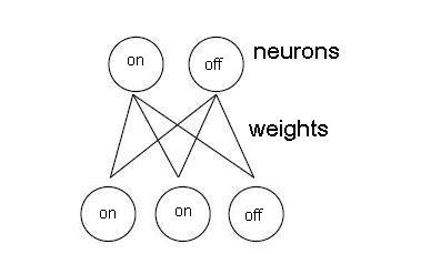
In a restricted Boltzmann Machine, every connection is between a visible unit and a hidden unit. This makes the states of the hidden units conditionally independent given a state of the visible units. Figure 2 in the paper, reproduced below, is an illustration of a Restricted Boltzmann Machine.
Pre-training step
The purpose of this step if to learn the (initial) weights for an adaptive, multi-layer, non-linear encoder network that transforms the input data vector [math]\displaystyle{ x }[/math] into its low-dimensional feature representation [math]\displaystyle{ \mathbf f(x|W) }[/math]. Indeed, the pretraining step should find a good region from which to start the subsequent fine-tuning step.
Modeling binary data
MNIST dataset contains binary images modeled here using Restricted Boltzmann Machines (RBM) <ref> Y. Freund and D. Haussler. Unsupervised learning of distributions on binary vectors using two layer networks. In Advances in Neural Information Processing Systems 4, pages 912–919, San Mateo, CA., 1992. Morgan Kaufmann </ref>, which are a type of stochastic recurrent neural network.
The visible stochastic binary input vector [math]\displaystyle{ \mathbf x }[/math] and hidden stochastic binary feature vector [math]\displaystyle{ \mathbf h }[/math] are modeled by products of conditional Bernoulli distributions:
Where [math]\displaystyle{ \sigma(z) = \frac{1}{1+exp(-z)} }[/math] is the logistic function and [math]\displaystyle{ \mathbf W_{ij} }[/math] is a symmetric interaction term between input [math]\displaystyle{ \mathbf i }[/math] and feature [math]\displaystyle{ \mathbf j }[/math], and [math]\displaystyle{ b_i\ and \ b_j }[/math] are biases.
The marginal distribution over visible vector [math]\displaystyle{ \mathbf x }[/math] is then:
Where [math]\displaystyle{ \mathbf E(x,h) }[/math] is an energy term defined as below:
Finally, the parameter update term to perform gradient ascent in the log-likelihood is
With [math]\displaystyle{ \mathbf \epsilon }[/math] being the learning rate, [math]\displaystyle{ \mathbf \lt .\gt _{data} }[/math] denoting the the frequency with which input [math]\displaystyle{ \mathbf i }[/math] and feature [math]\displaystyle{ \mathbf j }[/math] are on together when the features are being driven by the observed data from the training set, and [math]\displaystyle{ \mathbf \lt .\gt _{model} }[/math] being the expectation (corresponding to [math]\displaystyle{ \mathbf \lt .\gt _{data} }[/math]) with respect to the distribution defined by the model.
As computations for [math]\displaystyle{ \mathbf \lt .\gt _{model} }[/math] are difficult, the 1-step divergence algorithm is used to circumvent this burden <ref> G. E. Hinton. Training products of experts by minimizing contrastive divergence. Neural Computation, 14(8):1711–1800, 2002</ref>:
Where [math]\displaystyle{ \mathbf \lt .\gt _{recon} }[/math] is the frequency with which input [math]\displaystyle{ \mathbf i }[/math] and feature [math]\displaystyle{ \mathbf j }[/math] are on together after stochastically activating features and reconstructing binary data. A simplified version of the above equation is used as the learning rule for the biases.
Modeling real value data
By generalizing RBM's to exponential family distributions, Welling et. al. could model images with real-valued pixels by using visible units that have a Gaussian distribution whose mean is determined by the hidden units:
[math]\displaystyle{ p(x_i=x|h) = \frac{1}{\sqrt{2*\pi* \sigma_i}}exp(-\frac{(x-b_i-\sigma_i\Sigma_j{h_{j}w_{ij}})^2}{2\sigma_i^2}) }[/math]
[math]\displaystyle{ p(h=1|x)=\sigma(b_j+\Sigma_i{W_{ij}\frac{x_i}{\sigma_i}}) }[/math]
Greedy recursive pretraining
This greedy, layer-by-layer training can be repeated several times to learn a deep, hierarchical model in which each layer of features captures strong high-order correlations between the activities of features in the layer below:
1. Learn the parameters [math]\displaystyle{ \mathbf W^1 }[/math] of a Bernoulli or Gaussian model.
2. Freeze the parameters of the lower-level model and use the activation probabilities of the binary features, when they are being driven by training data, as the data for training the next layer of binary features.
3. Freeze the parameters [math]\displaystyle{ \mathbf W^2 }[/math] that define the second layer of features and use the activation probabilities of those features as data for training the third layer of features.
4. Proceed recursively for as many layers as desired.
Fine-tuning step
For fine-tuning model parameters using the NCA objective function (introduced above) the method of conjugate gradients is used. To determine an adequate number of epochs and avoid overfitting, only a fraction of the training data is used for fine-tuning, and then performance is tested on the remaining validation data.
Regularized Nonlinear NCA
In many applications, a large supply of unlabeled data is readily available but the amount of labeled data (which typically requires expert knowledge to produce), is very limited. In order to take advantage of the information in the unlabeled data to enhance nonlinear NCA performance, the regularized NCA framework is proposed. Once the pretarining step for individual RBM's is each level of the network is done, one can replace the stochastic activities of the binary features by deterministic, real-valued probabilities. This allows for backpropagating through the entire network to fine-tune the weights for optimal reconstruction of the data.
Performing such training step does not require labeled data and produces low-dimensional codes that are good at reconstructing the input data vectors, and tend to preserve class neighbourhood structure. Accordingly, a new objective function [math]\displaystyle{ C }[/math] is formulated combining NCA and autoencoder objective functions:
Where [math]\displaystyle{ \mathbf E }[/math] is the reconstruction error and [math]\displaystyle{ \mathbf \lambda }[/math] is a trade-off parameter.
For example assuming a semi-supervised learning setting, consider having a set of [math]\displaystyle{ \mathbf N_l }[/math] labeled training data [math]\displaystyle{ \mathbf (x^l,c^l) }[/math], and a set of [math]\displaystyle{ \mathbf N_u }[/math] unlabeled training data [math]\displaystyle{ \mathbf x^u }[/math]. The overall objective function would then be as below:
Where [math]\displaystyle{ \mathbf N=N_l+N_u }[/math] and [math]\displaystyle{ \mathbf E^n }[/math] is the reconstruction error for the input [math]\displaystyle{ \mathbf x^n }[/math].
Splitting codes into class-relevant and class-irrelevant parts
Accurate reconstruction of a digit image requires the code to contain information about aspects of the image such as its orientation, slant, size and stroke thickness. These aspects are not necessarily relevant to digit class may inevitably contribute to the Euclidean distance between codes and thus harm classification. To eliminate such unwanted effect, a 50-dimensional code is used, but only the first 30 dimensions are used in the NCA objective function calculations. The remaining 20 dimensions were free to code all those aspects of an image that do not affect its class label but are important for reconstruction, and are therefore used to compute the reconstruction errors.
Experiments
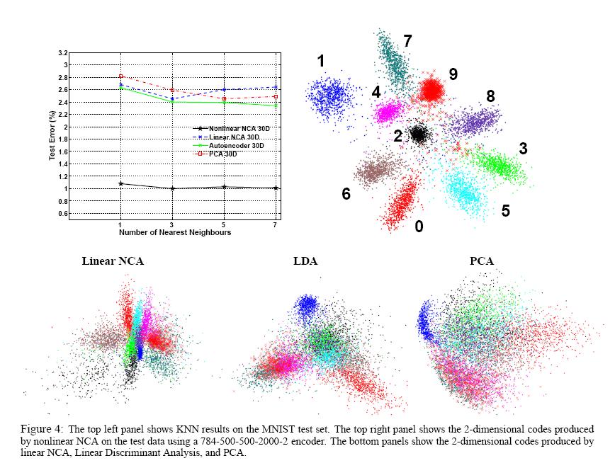
Experimental results presented for the MNIST dataset containing 60000 training and 10000 test images of 28x28 handwritten digits, show the superior performance of the proposed algorithm (i.e. nonlinear NCA). An 28x28-500-500-2000-30 architecture is used for the multi-layer neural network.
Obtained results show that nonlinear NCA achieves minimum error rate of 1.01% using 7 nearest neighbours. This compares favorably to the best reported error rates (without using any domain-specific knowledge) of 1.6% for randomly initialized backpropagation and 1.4% for Support Vector Machines.
Results also show that Regularized nonlinear NCA not only performs better than the nonlinear NCA on unlabeled data but also performs slightly better on labelled data.

Summary
It has been shown how to pretrain and fine-tune a deep nonlinear encoder network to learn a similarity metric over the input space facilitating nearest neighbor classification.
The method achieved the least error on a version of MINST handwritten digit recognition task without using any domain specific knowledge.
The classification accuracy is high even with the limited labeled training data.
References
<references/>

