regression on Manifold using Kernel Dimension Reduction

An Algorithm for finding a new linear map for dimension reduction.

Introduction

This paper <ref>[1] Jen Nilsson, Fei Sha, Michael I. Jordan, Regression on Manifold using Kernel Dimension Reduction, 2007 - cs.utah.edu </ref>introduces a new algorithm for discovering a manifold that best preserves the information relevant to a non-linear regression. The approach introduced by the authors involves combining the machinery of Kernel Dimension Reduction (KDR) with Laplacian Eigenmaps by optimizing the cross-covariance operators in kernel feature space.

Two main challenges that we usually come across in supervised learning are making a choice of manifold to represent the covariance vector and to choose a function to represent the boundary for classification (i.e. regression surface). As a result of these two complexities, most of the research in supervised learning has been focused on learning linear manifolds. The authors introduce a new algorithm that makes use of methodologies developed in Sufficient Dimension Reduction (SDR) and Kernel Dimension Reduction (KDR). The algorithm is called Manifold Kernel Dimension Reduction (mKDR).

Sufficient Dimension Reduction

The purpose of Sufficient Dimension Reduction (SDR) is to find a linear subspace S such that the response vector Y is conditionally independent of the covariate vector X. More specifically, let [math]\displaystyle{ (X,B_X) }[/math] and [math]\displaystyle{ (Y,B_Y) }[/math] be measurable spaces of covariates X and response variable Y. SDR aims to find a linear subspace [math]\displaystyle{ S \subset X }[/math] such that [math]\displaystyle{ S }[/math] contains as much predictive information about the response [math]\displaystyle{ Y }[/math] as the original covariate space. As seen before in (Fukumizu, K., Bach, F. R., & Jordan, M. I. (2004))<ref>Fukumizu, K., Bach, F. R., & Jordan, M. I. (2004):Kernel Dimensionality Reduction for Supervised Learning</ref> this can be written more formally as a conditional independence assertion.

[math]\displaystyle{ Y \perp B^T X | B^T X }[/math] [math]\displaystyle{ \Longleftrightarrow Y \perp (X - B^T X) | B^T X }[/math]. <ref>[2] Jen Nilsson, Fei Sha, Michael I. Jordan, Regression on Manifold using Kernel Dimension Reduction, 2007 - cs.utah.edu </ref>

The above statement says that [math]\displaystyle{ S \subset X }[/math] such that the conditional probability density function [math]\displaystyle{ p_{Y|X}(y|x)\, }[/math] is preserved in the sense that [math]\displaystyle{ p_{Y|X}(y|x) = p_{Y|B^T X}(y|b^T x)\, }[/math] for all [math]\displaystyle{ x \in X \, }[/math] and [math]\displaystyle{ y \in Y \, }[/math], where [math]\displaystyle{ B^T X\, }[/math] is the orthogonal projection of [math]\displaystyle{ X\, }[/math] onto [math]\displaystyle{ S\, }[/math]. The subspace [math]\displaystyle{ S\, }[/math] is referred to as a dimension reduction subspace. Note that [math]\displaystyle{ S\, }[/math] is not unique.

We can define a minimal subspace as the intersection of all dimension reduction subspaces [math]\displaystyle{ S\, }[/math]. However, a minimal subspaces will not necessarily satisfy the conditional independence assertion specified above. But when it does, it is referred to as the central subspace.

This is one of the primary goals of the method i.e. to find a central subspace. Several approaches have been introduced in the past, mostly based on inverse regression (Li, 1991)<ref>Sliced inverse regression for dimension reduction. Journal of the American Statistical Association, 86, 316–327</ref> (Li, 1992)<ref>On principal Hessian directions for data visualization and dimension reduction: Another application of Stein’s lemma. Journal of the American Statistical Association, 86, 316–342.</ref>. The main intuition behind this approach is to find [math]\displaystyle{ \mathbb{E[} X|Y \mathbb{]} }[/math] becuase if the the forward regression model [math]\displaystyle{ P(X|Y) }[/math] is concenterated in a subspace of [math]\displaystyle{ X }[/math], then [math]\displaystyle{ \mathbb{E[} X|Y \mathbb{]} }[/math] should also lie in [math]\displaystyle{ X }[/math] (See Li. 1991 for more details<ref>Sliced inverse regression for dimension reduction. Journal of the American Statistical Association, 86, 316–327</ref>). Unfortunately, such an approach proposes a difficulty of making strong assumptions on the distribution of X (e.g. the distribution should be elliptical) and the methods of inverse regression fail if such assumptions are not satisfied. In order to overcome this problem, the authors turn to the description of KDR, i.e. an approach to SDR which does not make such strong assumptions.

Kernel Dimension Reduction

The framework for Kernel Dimension Reduction was primarily described by Kenji Fukumizu <ref>Fukumizu, K., Bach, F. R., & Jordan, M. I. (2004). Dimensionality reduction for supervised learning with reproducing kernel Hilbert spaces. Journal of Machine Learning Research, 5, 73–99.</ref><ref>Fukumizu, K., Bach, F. R., & Jordan, M. I. (2006). Kernel dimension reduction in regression (Technical Report). Department of Statistics, University of California, Berkeley.</ref>. The key idea behind KDR is to map random variables X and Y to Reproducing Kernel Hilbert Spaces (RHKS). Before going ahead, we make some preliminary definitions.

---

[math]\displaystyle{ \mathbb{D} }[/math]:- Reproducing Kernel Hilbert Space A Hilbert space is a (possibly infinite dimension) inner product space that is a complete metric space. Elements of a Hilbert space may be functions. A reproducing kernel Hilbert space is a Hilbert space of functions on some set [math]\displaystyle{ T }[/math] such that there exists a function [math]\displaystyle{ K }[/math] (known as the reproducing kernel) on [math]\displaystyle{ T \times T }[/math], where for any [math]\displaystyle{ t \in T }[/math], [math]\displaystyle{ K( \cdot , t ) }[/math] is in the RKHS.

[math]\displaystyle{ \mathbb{D} }[/math]:- Cross-Covariance Operators Let [math]\displaystyle{ ({ H}_1, k_1) }[/math] and [math]\displaystyle{ ({H}_2, k_2) }[/math] be RKHS over [math]\displaystyle{ (\Omega_1, { B}_1) }[/math] and [math]\displaystyle{ (\Omega_2, {B}_2) }[/math], respectively, with [math]\displaystyle{ k_1 }[/math] and [math]\displaystyle{ k_2 }[/math] measurable. For a random vector [math]\displaystyle{ (X, Y) }[/math] on [math]\displaystyle{ \Omega_1 \times \Omega_2 }[/math]. Using the Reisz representation theorem, one may show that there exists a unique operator [math]\displaystyle{ \Sigma_{YX} }[/math] from [math]\displaystyle{ H_1 }[/math] to [math]\displaystyle{ H_2 }[/math] such that
[math]\displaystyle{ \lt g, \Sigma_{YX} f\gt _{H_2} = \mathbb{E}_{XY} [f(X)g(Y)] - \mathbb{E}[f(X)]\mathbb{E}[g(Y)] }[/math]
holds for all [math]\displaystyle{ f \in H_1 }[/math] and [math]\displaystyle{ g \in H_2 }[/math], which is called the cross-covariance operator.

[math]\displaystyle{ \mathbb{D} }[/math]:- Condtional Covariance Operators Let [math]\displaystyle{ (H_1, k_1) }[/math] and [math]\displaystyle{ (H_2, k_2) }[/math] be RKHS on [math]\displaystyle{ \Omega_1 \times \Omega_2 }[/math], and let [math]\displaystyle{ (X,Y) }[/math] be a random vector on measurable space [math]\displaystyle{ \Omega_1 \times \Omega_2 }[/math]. The conditonal cross-covariance operator of [math]\displaystyle{ (Y,Y) }[/math] given [math]\displaystyle{ X }[/math] is defined by
[math]\displaystyle{ \Sigma_{YY|x}: = \Sigma_{YY} - \Sigma_{YX}\Sigma_{XX}^{-1}\Sigma_{XY} }[/math].

[math]\displaystyle{ \mathbb{D} }[/math] :- Conditional Covariance Operators and Condtional Indpendence Let [math]\displaystyle{ (H_{11}, k_{11}) }[/math], [math]\displaystyle{ (H_{12},k_{12}) }[/math] and [math]\displaystyle{ (H_2, k_2) }[/math] be RKHS on measurable space [math]\displaystyle{ \Omega_{11} }[/math], [math]\displaystyle{ \Omega_{12} }[/math] and [math]\displaystyle{ \Omega_2 }[/math], respectively, with continuous and bounded kernels. Let [math]\displaystyle{ (X,Y)=(U,V,Y) }[/math] be a random vector on [math]\displaystyle{ \Omega_{11}\times \Omega_{12} \times \Omega_{2} }[/math], where [math]\displaystyle{ X = (U,V) }[/math], and let [math]\displaystyle{ H_1 = H_{11} \otimes H_{12} }[/math] be the dirct product. It is assume that [math]\displaystyle{ \mathbb{E}_{Y|U} [g(Y)|U= \cdot] \in H_{11} }[/math] and [math]\displaystyle{ \mathbb{E}_{Y|X} [g(Y)|X= \cdot] \in H_{1} }[/math] for all [math]\displaystyle{ g \in H_2 }[/math]. Then we have
[math]\displaystyle{ \Sigma_{YY|U} \ge \Sigma_{YY|X} }[/math],
where the inequality refers to the order of self-adjoint operators. Furthermore, if [math]\displaystyle{ H_2 }[/math] is probability-deremining,
[math]\displaystyle{ \Sigma_{YY|X} = \Sigma_{YY|U} \Leftrightarrow Y \perp X|U }[/math].
Therefore, the effective subspace S can be found by minimizing the following function:
[math]\displaystyle{ \min_S\quad \Sigma_{YY|U} }[/math],[math]\displaystyle{ s.t. \quad U = \Pi_S X }[/math].

Note here for
[math]\displaystyle{ \Sigma_{YY|U} \ge \Sigma_{YY|X} }[/math],
in the sense of operator, the inequality means the variance of [math]\displaystyle{ Y }[/math] given data [math]\displaystyle{ U }[/math] is bigger than the variance of [math]\displaystyle{ Y }[/math] given data [math]\displaystyle{ X }[/math], which makes sense that [math]\displaystyle{ U }[/math] is just a part of the whole data [math]\displaystyle{ X }[/math].

---

Now that we have defined cross-covariance operators, we are finally ready to link the cross covariance operators to the central subspace. Consider any subspace [math]\displaystyle{ S \in X }[/math]. Then we can map this subspace to a RKHS [math]\displaystyle{ H_S }[/math] with a kernel function [math]\displaystyle{ K_S }[/math]. Furthermore, we define the conditional cross covariance operator as [math]\displaystyle{ \Sigma_{YY|S} }[/math] as if we were to regress [math]\displaystyle{ Y }[/math] on [math]\displaystyle{ S }[/math]. Then, intuitively, the residual error from [math]\displaystyle{ \Sigma_{YY|S} }[/math] should be greater than that from [math]\displaystyle{ \Sigma_{YY|S} }[/math]. Fukumizu etl al. (2006) <ref>Fukumizu, K., Bach, F. R., & Jordan, M. I. (2006). Kernel dimension reduction in regression (Technical Report). Department of Statistics, University of California, Berkeley.</ref> formalized that it would be trues unless [math]\displaystyle{ S }[/math] contains the central subspace. The intuition is formalized in the following theorem.

[math]\displaystyle{ \mathfrak{Theorem 1:-} }[/math] Suppose [math]\displaystyle{ Z = B^T B X \in S }[/math] where [math]\displaystyle{ B \in \mathbb{R}^{D \times d} }[/math] is a projection matrix such that [math]\displaystyle{ B^T B }[/math] is an identity matrix. Further assume Gaussian RBF kernels for [math]\displaystyle{ K_X, K_Y, and K_S }[/math]. Then

-) [math]\displaystyle{ \Sigma_{YY|X} \prec \Sigma_{YY|Z} }[/math] where [math]\displaystyle{ \prec }[/math] stands for "less than or equal to" in some operator partial ordering.

-) [math]\displaystyle{ \Sigma_{YY|X} = \Sigma_{YY|Z} }[/math] if and only if [math]\displaystyle{ Y \bot (X - B^T X)|B^T X }[/math], that is, [math]\displaystyle{ S }[/math] is a central subspace

One thing to note about the theorem specifically is that it doesn't impose any strong assumptions on the distribution of X, Y or their marginal distribution [math]\displaystyle{ \mathbb{P} }[/math](Y|X). (See Fukumizu et. al. 2006). This theorem leads to the new algorithm for estimating the central subspace characterized by B. Let [math]\displaystyle{ \{x_i,y_i\}_{i=1}^{N} }[/math] denote the N samples from the joint distribution of [math]\displaystyle{ \mathbb{P} }[/math](X, Y) and let [math]\displaystyle{ K_Y \in \mathbb{R}^{N \times N} }[/math] and [math]\displaystyle{ K_Z \in \mathbb{R}^{N \times N} }[/math] denote the Gram matrices comuted over y_i and z_i = B^T x_i}. Then Fukumizu et al. (2006) <ref>Fukumizu, K., Bach, F. R., & Jordan, M. I. (2006). Kernel dimension reduction in regression (Technical Report). Department of Statistics, University of California, Berkeley.</ref> show that this problem can be formulated as

[math]\displaystyle{ \min Tr \mathbb{[}K_Y^C(K_Z^C + N \in I^{-1}) \mathbb{]} }[/math] such that [math]\displaystyle{ B^T B = I }[/math]

where I is the Identity matrix and [math]\displaystyle{ \epsilon }[/math] is a regularization coefficient. The matrix K^C denotes the centered kernel matrices

[math]\displaystyle{ K^c = \left(I - \frac{1}{N}ee^T \right) K\left(I - \frac{1}{N}ee^T \right) }[/math]

where e is a vector of all ones.

Manifold Learning

Let [math]\displaystyle{ \{x_i,y_i\}_{i=1}^{N} }[/math] denote N data points sampled from the submanifold. Laplacian eigenmaps also appeal to a simple geometric intuition: namely, that nearby high dimensional inputs should be mapped to nearby low dimensional outputs. To this end, a positive weight W_ij is associated with inputs x_i and x_j if either input is among the other’s k-nearest neighbors. Usually, the values of the weights are either chosen to be constant, say Wij = 1/k, or exponentially decaying, as [math]\displaystyle{ W_{ij} = exp \left(\frac{- \|x_i - x_j \|^2}{\sigma^2}\right) }[/math]. Let D denote the diagonal matrix with elements [math]\displaystyle{ D_{ii} = \sum_{\forall j}W_{ij} }[/math]. Then the outputs y_i can be chosen such that it minimizes the cost function:

[math]\displaystyle{ \Psi(Y) = \sum_{\forall ij} \frac{W_ij\|y_i - y_j \|^2}{\sqrt{D_{ii}D_{jj}}} }[/math] (6)

The embedding is computed from the bottom eigenvectors of the matrix [math]\displaystyle{ \Psi = I - D^{- \frac{1}{2}} W D^{- \frac{1}{2}} }[/math] where the matrix [math]\displaystyle{ \Psi }[/math] is a symmetrized, normalized form of the graph Laplacian, given by D - W.

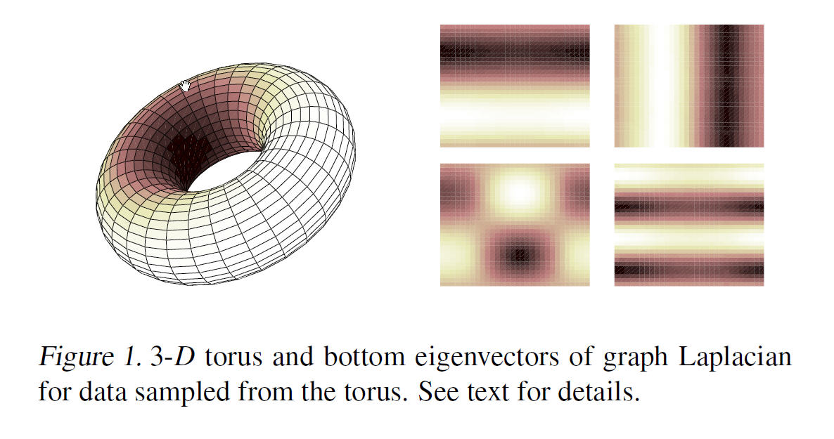
As an example, the figure below shows some of the first non-constant eigenvectors (mapped onto 2-D) for data points sampled from a 3-D torus. The image intesities correspond to high and low values of the eigen vectors. The variation in the intensities can be interpreted as the high and low frequency components of the harmonic functions. Intuitively, these eigenvectors can be used to approximate smooth functions on the manifold.

Manifold Kernel Dimension Reduction

The new algorithm introduced by the authors is called Manifold Kernal Dimension Reduction (mKDR) which combines ideas from supervised manifold learning and Kernel Dimension Reduction.

In essence the algorithm is has three main elements:

(1) Compute a Low-Dimension embedding of the covariates X; (2) Parametrize the central subspace as a linear transformation of the lower-dimensional embedding; (3) Compute the coefficients of the optimal linear map using the Kernel Dimension Reduction framework

The linear map achieved from the algorithm yields directions in the low-dimensional embedding that contribute most significantly to the central subspace. the authors start by illustrating the derivation of the algorithm and then outline the mKDR algorithm.

Derivation

From an M-Dimensional embedding [math]\displaystyle{ U \in \mathcal{U} \subset \mathbb{R}^{M \times N} }[/math] choose M eigenvectors [math]\displaystyle{ \{v_m\}_{m=1}^{M} }[/math] (see below for a choice of M).Then continuing from the KDR framework, consider a Kernel function that maps a point B^Tx_i in the central subspace to the Reproducing Kernel Hilbert Space (RKHS). Construct the mapping K(;) as

[math]\displaystyle{ K \left(; B^T x_i \right) \approx \Phi u_i }[/math]

where [math]\displaystyle{ \Phi u_i }[/math] is a linear expression approximating the Kernel Function. Note that, [math]\displaystyle{ \Phi \in \mathbb{R}^{M \times M} }[/math] is a linear map independent of x_i and our aim now is to find [math]\displaystyle{ \Phi }[/math]. This can be done through the KDR framework by minimizing the cost function [[Tr [math]\displaystyle{ \mathbb{[} K_Y^C(K_Z^C + N \in I) \mathbb{]} }[/math]]] for statistical independence between y_i and x_i. Then the Gram Matrix is approximated and parametrized by the linear map [math]\displaystyle{ \Phi }[/math] i.e.

[math]\displaystyle{ \lt K(;B^T x_i),K(B^T x_j)\gt \approx u_i^T \Phi^T \Phi u_j }[/math]

Define [math]\displaystyle{ \Omega = \Phi^T \Phi }[/math]. Then continuing from

[math]\displaystyle{ }[/math]

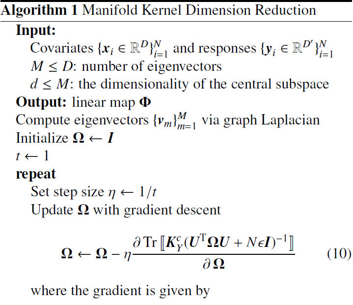
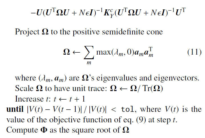
Algorithm

Experimental Results

Regression on Tours

In this section we analyze data points lying on the surface of a torus, illustrated in Fig. 1. A torus can be constructed by rotating a 2-D cycle in [math]\displaystyle{ R^3 }[/math] with respect to an axis. Hence giving any data point on the surface two degrees of freedom: the rotated angle [math]\displaystyle{ \theta_r }[/math] with respect to the axis and the polar angle [math]\displaystyle{ \theta_p }[/math] on the cycle. Our synthesized data set is formed by sampling these two angles from the Cartesian product [math]\displaystyle{ [0 2\pi] × [0 2\pi] }[/math]. As a result of that the 3-D coordinates of our torus will be [math]\displaystyle{ \mathbf{x_1=(2+cos\theta_r)cos\theta_p, x_2=(2+cos\theta_r)sin\theta_p} }[/math] and [math]\displaystyle{ \mathbf{x_3=sin\theta_r} }[/math]. After that we embed the torus in [math]\displaystyle{ \mathbf{x \in R^{10}} }[/math] by augmenting the coordinates with 7-dimensional all-zero or random vectors. For setting up the regression problem, we define the response by [math]\displaystyle{ \mathbf{y=\sigma[-17(\sqrt((\theta_r-\pi)^2+(\theta_p-\pi)^2)-0.6\pi)]} }[/math] where [math]\displaystyle{ \sigma[.] }[/math] is the sigmoid function. The colors on the surface of the torus in Fig. 1 correspond to the value of the response.

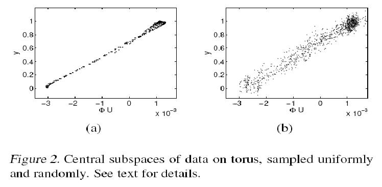
The mKDR was applied to the torus data set generated from 961 uniformly sampled angles [math]\displaystyle{ \theta_p }[/math] and [math]\displaystyle{ \theta_r }[/math] and [math]\displaystyle{ M = 50 }[/math] bottom eigenvectors from the graph Laplacian were used. The mKDR algorithm then computed the matrix [math]\displaystyle{ \mathbf{ \Phi \in R^{50 \times 50}} }[/math] that minimizes the empirical conditional covariance operator; This matrix turned out to be of nearly rank 1 and can be approximated by [math]\displaystyle{ \mathbf{a^T a} }[/math] where [math]\displaystyle{ \mathbf{a} }[/math] is the eigenvector corresponding to the largest eigenvalue. Hence, we projected the 50-D embedding of the graph Laplacian onto this principal direction [math]\displaystyle{ \mathbf{a} }[/math].

[math]\displaystyle{ \mathbf{a^T a} }[/math] <This section will be updated in near future.>

Further Research

This paper presented a new algorithm for dimensionality reduction that is appropriate when supervised information is available. The algorithm stands out not only because of its higher predictive power, but also because it combines the ideas from two strands of research i.e. Sufficient Dimension Reduction from Statistics and Manifold Learning from the Machine Learning literature. The ideas from two diverse fields is essentially connected by the ideas proposed in the methodology of Kernel Dimension Reduction.

As illustrated in the examples above, the algorithm finds a lower dimension and predictive subspaces and revealed some interesting patterns. Overall, the mKDR algorithm is a particular instantiation of the framework of kernel dimension reduction. Thus, it inherits all the advantages of the kernel methods in general, including the abuility to handle multivariate response variables and non-vectorial data.

References

(this section will be updated shortly)