Training And Inference with Integers in Deep Neural Networks
Introduction
Deep neural networks have enjoyed much success in all manners of tasks, but it is common for these networks to be complicated and have high memory requirements while performing many floating-point operations (FLOPs). As a result, running many of these models will be very expensive in terms of energy use, and using state-of-the-art networks in applications where energy is limited can be very difficult. In order to overcome this and allow use of these networks in situations with low energy availability, the energy costs must be reduced while trying to maintain as high network performance as possible and/or practical.
Most existing methods focus on reducing the energy requirements during inference rather than training. Since training with SGD requires accumulation, training usually has higher precision demand than inference. Most of the existing methods focus on how to compress a model for inference, rather than during training. This paper proposes a framework to reduce complexity both during training and inference through the use of integers instead of floats. The authors address how to quantize all operations and operands as well as examining the bitwidth requirement for SGD computation & accumulation. Using integers instead of floats results in energy-savings because integer operations are more efficient than floating point (see the table below). Also, there already exists dedicated hardware for deep learning that uses integer operations (such as the 1st generation of Google TPU) so understanding the best way to use integers is well-motivated. A TPU is a Tensor Processing Unit developed by Google for Tensor operations. TPU is comparative to a GPU but produces higher IO per second for low precision computations.
| Energy(pJ) | Area([math]\displaystyle{ \mu m^2 }[/math]) | |||
|---|---|---|---|---|
| Operation | MUL | ADD | MUL | ADD |
| 8-bit INT | 0.2 | 0.03 | 282 | 36 |
| 16-bit FP | 1.1 | 0.4 | 1640 | 1360 |
| 32-bit FP | 3.7 | 0.9 | 7700 | 4184 |
The authors call the framework WAGE because they consider how best to handle the Weights, Activations, Gradients, and Errors separately.
Related Work
Weight and Activation
Existing works to train DNNs on binary weights and activations [2] add noise to weights and activations as a form of regularization. The use of high-precision accumulation is required for SGD optimization since real-valued gradients are obtained from real-valued variables. XNOR-Net [11] uses bitwise operations to approximate convolutions in a highly memory-efficient manner, and applies a filter-wise scaling factor for weights to improve performance. However, these floating-point factors are calculated simultaneously during training, which aggravates the training effort. Ternary weight networks (TWN) [3] and Trained ternary quantization (TTQ)[9] offer more expressive ability than binary weight networks by constraining the weights to be ternary-valued {-1,0,1} using two symmetric thresholds. Tang et al.[14] achieve impressive results by using a binarization scheme according to which floating-point activation vectors are approximated as linear combinations of binary vectors, where the weights in the linear combination are floating-point. Still other approaches rely on relative quantization[13]; however, an efficient implementation is difficult to apply in practice due to the requirements of persisting and applying a codebook.
Gradient Computation and Accumulation
The DoReFa-Net quantizes gradients to low-bandwidth floating point numbers with discrete states in the backwards pass. In order to reduce the overhead of gradient synchronization in distributed training the TernGrad method quantizes the gradient updates to ternary values. In both works the weights are still stored and updated with float32, and the quantization of batch normalization and its derivative is ignored.
WAGE Quantization
The core idea of the proposed method is to constrain the following to low-bitwidth integers on each layer:
- W: weight in inference
- a: activation in inference
- e: error in backpropagation
- g: gradient in backpropagation
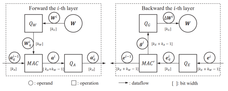
We extend the original definition of errors to multi-layer: error e is the gradient of activation a for the perspective of each convolution or fully-connected layer, while gradient g particularly refers to the gradient accumulation of weight W. Considering the i-th layer of a feed-forward network.
The error and gradient are defined as:
[math]\displaystyle{ e^i = \frac{\partial L}{\partial a^i}, g^i = \frac{\partial L}{\partial W^i} }[/math]
where L is the loss function.
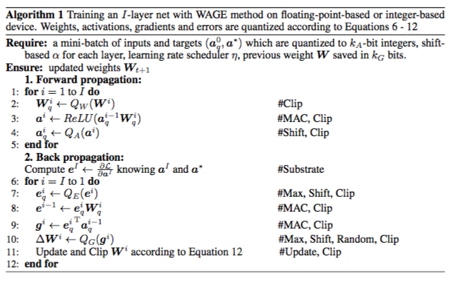
The precision in bits of the errors, activations, gradients, and weights are [math]\displaystyle{ k_E }[/math], [math]\displaystyle{ k_A }[/math], [math]\displaystyle{ k_G }[/math], and [math]\displaystyle{ k_W }[/math] respectively. As shown in the above figure, each quantity also has a quantization operators to reduce bitwidth increases caused by multiply-accumulate (MAC) operations. Also, note that since this is a layer-by-layer approach, each layer may be followed or preceded by a layer with different precision, or even a layer using floating point math.
Shift-Based Linear Mapping and Stochastic Mapping
The proposed method makes use of a linear mapping where continuous, unbounded values are discretized for each bitwidth [math]\displaystyle{ k }[/math] with a uniform spacing of
[math]\displaystyle{ \sigma(k) = 2^{1-k}, k \in Z_+ }[/math] With this, the full quantization function is
[math]\displaystyle{ Q(x,k) = Clip\left \{ \sigma(k) \cdot round\left [ \frac{x}{\sigma(k)} \right ], -1 + \sigma(k), 1 - \sigma(k) \right \} }[/math],
where [math]\displaystyle{ round }[/math] approximates continuous values to their nearest discrete state, and [math]\displaystyle{ Clip }[/math] is the saturation function that clips unbounded values to [math]\displaystyle{ [-1 + \sigma, 1 - \sigma] }[/math]. Note that this function is only using when simulating integer operations on floating-point hardware, on native integer hardware, this is done automatically. In addition to this quantization function, a distribution scaling factor is used in some quantization operators to preserve as much variance as possible when applying the quantization function above. The scaling factor is defined below.
[math]\displaystyle{ Shift(x) = 2^{round(log_2(x))} }[/math]
Finally, stochastic rounding is substituted for small or real-valued updates during gradient accumulation.
A visual representation of these operations is below.

Weight Initialization
In this work, batch normalization is simplified to a constant scaling layer in order to sidestep the problem of normalizing outputs without floating point math, and to remove the extra memory requirement with batch normalization. As such, some care must be taken when initializing weights. The authors use a modified initialization method base on MSRA[4].
[math]\displaystyle{ W \thicksim U(-L, +L),L = max \left \{ \sqrt{6/n_{in}}, L_{min} \right \}, L_{min} = \beta \sigma }[/math]
[math]\displaystyle{ n_{in} }[/math] is the layer fan-in number, [math]\displaystyle{ U }[/math] denotes uniform distribution. The original initialization method for [math]\displaystyle{ \eta }[/math] is modified by adding the condition that the distribution width should be at least [math]\displaystyle{ \beta \sigma }[/math], where [math]\displaystyle{ \beta }[/math] is a constant greater than 1 and [math]\displaystyle{ \sigma }[/math] is the minimum step size seen already. This prevents weights being initialised to all-zeros in the case where the bitwidth is low, or the fan-in number is high.
Quantization Details
Weight [math]\displaystyle{ Q_W(\cdot) }[/math]
[math]\displaystyle{ W_q = Q_W(W) = Q(W, k_W) }[/math]
The quantization operator is simply the quantization function previously introduced.
Activation [math]\displaystyle{ Q_A(\cdot) }[/math]
The authors say that the variance of the weights passed through this function will be scaled compared to the variance of the weights as initialized. To prevent this effect from blowing up the network outputs, they introduce a scaling factor [math]\displaystyle{ \alpha }[/math]. Notice that it is constant for each layer.
[math]\displaystyle{ \alpha = max \left \{ Shift(L_{min} / L), 1 \right \} }[/math]
The quantization operator is then
[math]\displaystyle{ a_q = Q_A(a) = Q(a/\alpha, k_A) }[/math]
The scaling factor approximates batch normalization.
Error [math]\displaystyle{ Q_E(\cdot) }[/math]
The magnitude of the error can vary greatly, and that a previous approach (DoReFa-Net[5]) solves the issue by using an affine transform to map the error to the range [math]\displaystyle{ [-1, 1] }[/math], apply quantization, and then applying the inverse transform. However, the authors claim that this approach still requires using float32, and that the magnitude of the error is unimportant: rather it is the orientation of the error. Thus, they only scale the error distribution to the range [math]\displaystyle{ \left [ -\sqrt2, \sqrt2 \right ] }[/math] and quantise:
[math]\displaystyle{ e_q = Q_E(e) = Q(e/Shift(max\{|e|\}), k_E) }[/math]
Max is the element-wise maximum. Note that this discards any error elements less than the minimum step size.
Gradient [math]\displaystyle{ Q_G(\cdot) }[/math]
Similar to the activations and errors, the gradients are rescaled:
[math]\displaystyle{ g_s = \eta \cdot g/Shift(max\{|g|\}) }[/math]
[math]\displaystyle{ \eta }[/math] is a shift-based learning rate. It is an integer power of 2. The shifted gradients are represented in units of minimum step sizes [math]\displaystyle{ \sigma(k) }[/math]. When reducing the bitwidth of the gradients (remember that the gradients are coming out of a MAC operation, so the bitwidth may have increased) stochastic rounding is used as a substitute for small gradient accumulation.
[math]\displaystyle{ \Delta W = Q_G(g) = \sigma(k_G) \cdot sgn(g_s) \cdot \left \{ \lfloor | g_s | \rfloor + Bernoulli(|g_s| - \lfloor | g_s | \rfloor) \right \} }[/math]
This randomly rounds the result of the MAC operation up or down to the nearest quantization for the given gradient bitwidth. The weights are updated with the resulting discrete increments:
[math]\displaystyle{ W_{t+1} = Clip \left \{ W_t - \Delta W_t, -1 + \sigma(k_G), 1 - \sigma(k_G) \right \} }[/math]
Miscellaneous
To train WAGE networks, the authors used pure SGD exclusively because more complicated techniques such as Momentum or RMSProp increase memory consumption and are complicated by the rescaling that happens within each quantization operator.
The quantization and stochastic rounding are a form of regularization.
The authors didn't use a traditional softmax with cross-entropy loss for the experiments because there does not yet exist a softmax layer for low-bit integers. Instead, they use a sum of squared error loss. This works for tasks with a small number of categories, but does not scale well.
Experiments
For all experiments, the default layer bitwidth configuration is 2-8-8-8 for Weights, Activations, Gradients, and Error bits. The weight bitwidth is set to 2 because that results in ternary weights, and therefore no multiplication during inference. They authors argue that the bitwidth for activation and errors should be the same because the computation graph for each is similar and might use the same hardware. During training, the weight bitwidth is 8. For inference the weights are ternarized.
Implementation Details
MNIST: Network is LeNet-5 variant[6] with 32C5-MP2-64C5-MP2-512FC-10SSE.
SVHN & CIFAR10: VGG variant[7] with 2×(128C3)-MP2-2×(256C3)-MP2-2×(512C3)-MP2-1024FC-10SSE. For CIFAR10 dataset, the data augmentation is followed in Lee et al. (2015)[10] for training.
ImageNet: AlexNet variant[8] on ILSVRC12 dataset.
| Method | [math]\displaystyle{ k_W }[/math] | [math]\displaystyle{ k_A }[/math] | [math]\displaystyle{ k_G }[/math] | [math]\displaystyle{ k_E }[/math] | Opt | BN | MNIST | SVHN | CIFAR10 | ImageNet |
|---|---|---|---|---|---|---|---|---|---|---|
| BC | 1 | 32 | 32 | 32 | Adam | yes | 1.29 | 2.30 | 9.90 | |
| BNN | 1 | 1 | 32 | 32 | Adam | yes | 0.96 | 2.53 | 10.15 | |
| BWN | 1 | 32 | 32 | 32 | withM | yes | 43.2/20.6 | |||
| XNOR | 1 | 1 | 32 | 32 | Adam | yes | 55.8/30.8 | |||
| TWN | 2 | 32 | 32 | 32 | withM | yes | 0.65 | 7.44 | 34.7/13.8 | |
| TTQ | 2 | 32 | 32 | 32 | Adam | yes | 6.44 | 42.5/20.3 | ||
| DoReFa | 8 | 8 | 32 | 8 | Adam | yes | 2.30 | 47.0/ | ||
| TernGrad | 32 | 32 | 2 | 32 | Adam | yes | 14.36 | 42.4/19.5 | ||
| WAGE | 2 | 8 | 8 | 8 | SGD | no | 0.40 | 1.92 | 6.78 | 51.6/27.8 |
Training Curves and Regularization
The authors compare the 2-8-8-8 WAGE configuration introduced above, a 2-8-f-f (meaning float32) configuration, and a completely floating point version on CIFAR10. The test error is plotted against epoch. For training these networks, the learning rate is divided by 8 at the 200th epoch and again at the 250th epoch.
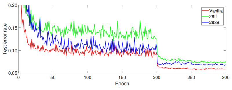
The convergence of the 2-8-8-8 has comparable convergence to the vanilla CNN and outperforms the 2-8-f-f variant. The authors speculate that this is because the extra discretization acts as a regularizer.
Bitwidth of Errors
The CIFAR10 test accuracy is plotted against bitwidth below and the error density for a single layer is compared with the Vanilla network.
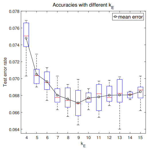
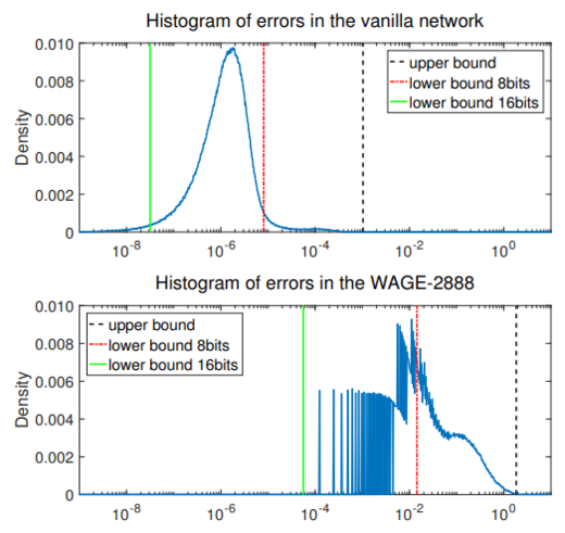
The table below shows the test error rates on CIFAR10 when left-shift upper boundary with factor γ. From this table we could see that large values play critical roles for backpropagation training even though they are infrequent while the majority with small values are just noise.

Bitwidth of Gradients
The authors next investigated the choice of a proper [math]\displaystyle{ k_G }[/math] for gradients using the CIFAR10 dataset.
| [math]\displaystyle{ k_G }[/math] | 2 | 3 | 4 | 5 | 6 | 7 | 8 | 9 | 10 | 11 | 12 |
|---|---|---|---|---|---|---|---|---|---|---|---|
| error | 54.22 | 51.57 | 28.22 | 18.01 | 11.48 | 7.61 | 6.78 | 6.63 | 6.43 | 6.55 | 6.57 |
The results show similar bitwidth requirements as the last experiment for [math]\displaystyle{ k_E }[/math].
The authors also examined the effect of bitwidth on the ImageNet implementation.
Here, C denotes 12 bits (Hexidecimal) and BN refers to batch normalization being added. 7 models are used: 2888 from the first experiment, 288C for more accurate errors (12 bits), 28C8 for larger buffer space, 28f8 for non-quantization of gradients, 28ff for errors and gradients in float32, and 28ff with BN added. The baseline vanilla model refers to the original AlexNet architecture.
| Pattern | vanilla | 28ff-BN | 28ff | 28f8 | 28C8 | 288C | 2888 |
|---|---|---|---|---|---|---|---|
| error | 19.29 | 20.67 | 24.14 | 23.92 | 26.88 | 28.06 | 27.82 |
The comparison between 28C8 and 288C shows that the model may perform better if it has more buffer space [math]\displaystyle{ k_G }[/math] for gradient accumulation than if it has high-resolution orientation [math]\displaystyle{ k_E }[/math]. The authors also noted that batch normalization and [math]\displaystyle{ k_G }[/math] are more important for ImageNet because the training set samples are highly variant.
Discussion
The authors have a few areas they believe this approach could be improved.
MAC Operation: The 2-8-8-8 configuration was chosen because the low weight bitwidth means there aren't any multiplication during inference. However, this does not remove the requirement for multiplication during training. 2-2-8-8 configuration satisfies this requirement, but it is difficult to train and detrimental to the accuracy.
Non-linear Quantization: The linear mapping used in this approach is simple, but there might be a more effective mapping. For example, a logarithmic mapping could be more effective if the weights and activations have a log-normal distribution.
Normalization: Normalization layers (softmax, batch normalization) were not used in this paper. Quantized versions are an area of future work
Conclusion
A framework for training and inference without the use of floating-point representation is presented. By quantizing all operations and operands of a network, the authors successfully reduce the energy costs of both training and inference with deep learning architectures. Future work may further improve compression and memory requirements.
Implementation
The following repository provides the source code for the paper: https://github.com/boluoweifenda/WAGE. The repository provides the source code as written by the authors, in Tensorflow.
Limitation
- The paper states the advantages in energy costs, but is there any limitation or trade-off by selecting integer instead of float-point-operation? What is a good situation for such implementation? The authors should explain more on this.
References
- Sze, Vivienne; Chen, Yu-Hsin; Yang, Tien-Ju; Emer, Joel (2017-03-27). "Efficient Processing of Deep Neural Networks: A Tutorial and Survey". arXiv:1703.09039 [cs].
- Courbariaux, Matthieu; Bengio, Yoshua; David, Jean-Pierre (2015-11-01). "BinaryConnect: Training Deep Neural Networks with binary weights during propagations". arXiv:1511.00363 [cs].
- Li, Fengfu; Zhang, Bo; Liu, Bin (2016-05-16). "Ternary Weight Networks". arXiv:1605.04711 [cs].
- He, Kaiming; Zhang, Xiangyu; Ren, Shaoqing; Sun, Jian (2015-02-06). "Delving Deep into Rectifiers: Surpassing Human-Level Performance on ImageNet Classification". arXiv:1502.01852 [cs].
- Zhou, Shuchang; Wu, Yuxin; Ni, Zekun; Zhou, Xinyu; Wen, He; Zou, Yuheng (2016-06-20). "DoReFa-Net: Training Low Bitwidth Convolutional Neural Networks with Low Bitwidth Gradients". arXiv:1606.06160 [cs].
- Lecun, Y.; Bottou, L.; Bengio, Y.; Haffner, P. (November 1998). "Gradient-based learning applied to document recognition". Proceedings of the IEEE. 86 (11): 2278–2324. doi:10.1109/5.726791. ISSN 0018-9219.
- Simonyan, Karen; Zisserman, Andrew (2014-09-04). "Very Deep Convolutional Networks for Large-Scale Image Recognition". arXiv:1409.1556 [cs].
- Krizhevsky, Alex; Sutskever, Ilya; Hinton, Geoffrey E (2012). Pereira, F.; Burges, C. J. C.; Bottou, L.; Weinberger, K. Q., eds. Advances in Neural Information Processing Systems 25 (PDF). Curran Associates, Inc. pp. 1097–1105.
- Chenzhuo Zhu, Song Han, Huizi Mao, and William J Dally. Trained ternary quantization. arXiv preprint arXiv:1612.01064, 2016.
- Chen-Yu Lee, Saining Xie, Patrick Gallagher, Zhengyou Zhang, and Zhuowen Tu. Deeplysupervisednets. In Artificial Intelligence and Statistics, pp. 562–570, 2015.
- Mohammad Rastegari, Vicente Ordonez, Joseph Redmon, and Ali Farhadi. Xnor-net: Imagenet classification using binary convolutional neural networks. In European Conference on Computer Vision, pp. 525–542. Springer, 2016.
- “Boluoweifenda/WAGE.” GitHub, github.com/boluoweifenda/WAGE.
- Han, S., Mao, H., & Dally, W. J. (2015). Deep compression: Compressing deep neural networks with pruning, trained quantization and huffman coding. arXiv preprint arXiv:1510.00149.
- Tang, Wei, Gang Hua, and Liang Wang. "How to train a compact binary neural network with high accuracy?." AAAI. 2017.