Multi-scale Dense Networks for Resource Efficient Image Classification
Introduction
Multi-Scale Dense Networks, MSDNets, are designed to address the growing demand for efficient object recognition. The issue with existing recognition networks is that they are either efficient networks, but don't do well on hard examples, or large networks that do well on all examples but require a large amount of resources. For example, the winner of the COCO 2016 competition was an ensemble of CNNs, which are likely far too resource-heavy to be used in any resource-limited application.
Note:
- There are two kinds of efficiency in this context, computational efficiency and resource efficiency.
- There are multiple cases for hard examples, such as large number of classification label, randomly blocked or zoomed images, or even complicated background that makes image recognition even more difficult.
In order to be efficient on all difficulties MSDNets propose a structure that can accurately output classifications for varying levels of computational requirements. The two cases that are used to evaluate the network are:
- Anytime Prediction: What is the best prediction the network can provide when suddenly prompted?
- Budget Batch Predictions: Given a maximum amount of computational resources, how well does the network do on the batch?
Related Networks
Computationally Efficient Networks
Much of the existing work on convolution networks that are computationally efficient at test time focus on reducing model size after training. Many existing methods for refining an accurate network to be more efficient include weight pruning [3,4,5], quantization of weights [6,7] (during or after training), and knowledge distillation [8,9], which trains smaller student networks to reproduce the output of a much larger teacher network. The proposed work differs from these approaches as it trains a single model which trades computation efficiency for accuracy at test time without re-training or finetuning.
Resource Efficient Networks
Unlike the above, resource efficient concepts consider limited resources as a part of the structure/loss. Examples of work in this area include:
- Efficient variants to existing state of the art networks
- Gradient boosted decision trees, which incorporate computational limitations into the training
- Fractal nets
- Adaptive computation time method
Related architectures
MSDNets pull on concepts from a number of existing networks:
- Neural fabrics and others, are used to quickly establish a low resolution feature map, which is integral for classification.
- Deeply supervised nets, introduced the incorporation of multiple classifiers throughout the network. (For example, a Branchynet (Teerapittayanon et al., 2016) is a deeply supervised network explicitly designed for efficiency. A Branchynet has multiple exit branches at various depths, each leading to a softmax classifier. At test time, if a classifier on an early exit branch makes a confident prediction, the rest of network need not be evaluated. However, unlike in MSDnets, in Branchynets early classifiers to not have access to low-resolution features. )
- The feature concatenation method from DenseNets(Dense net is CNN with shorter connections close to input and output) allows the later classifiers to not be disrupted by the weight updates from earlier classifiers.
Problem Setup
The authors consider two settings that impose computational constraints at prediction time.
Anytime Prediction
In the anytime prediction setting (Grubb & Bagnell, 2012), there is a finite computational budget [math]\displaystyle{ B \gt 0 }[/math] available for each test example [math]\displaystyle{ x }[/math]. Once the budget is exhausted, the prediction for the class is output using early exit. The budget is nondeterministic and varies per test instance. They assume that the budget is drawn from some joint distribution [math]\displaystyle{ P(x,B) }[/math]. They denote the loss of a model [math]\displaystyle{ f(x) }[/math] that has to produce a prediction for instance x with a budget of [math]\displaystyle{ B }[/math] by [math]\displaystyle{ L(f(x),B) }[/math]. The goal of the anytime learner is to minimize the expected loss under the budget distribution [math]\displaystyle{ L(f)=\mathop{\mathbb{E}}[L(f(x),B)]_{P(x,B)} }[/math].
Budgeted Batch Classification
In the budgeted batch classification setting, the model needs to classify a set of examples [math]\displaystyle{ D_{test} = {x_1, . . . , x_M} }[/math] within a finite computational budget [math]\displaystyle{ B \gt 0 }[/math] that is known in advance. The learner aims to minimize the loss across all examples in the [math]\displaystyle{ D_{test} }[/math], within a cumulative cost bounded by [math]\displaystyle{ B }[/math], which is denoted as [math]\displaystyle{ L(f(D_{test}),B) }[/math] for some suitable loss function [math]\displaystyle{ L }[/math].
Multi-Scale Dense Networks
Two solutions to the problems mentioned above:
- Train multiple networks of increasing capacity, and evaluate them at test time.
- Anytime setting: the evaluation can be stopped at any time point and return the most recent prediction
- Batch setting: the evaluation is stopped with no continuous training when the network is good enough.
- Build a deep network with a cascade of classifiers operating on the features of internal layers.
Integral Contributions
The way MSDNets aims to provide efficient classification with varying computational costs is to create one network that outputs results at depths. While this may seem trivial, as intermediate classifiers can be inserted into any existing network, two major problems arise.
Coarse Level Features Needed For Classification
The term coarse level feature refers to a set of filters in a CNN with low resolution. There are several ways to create such features. These methods are typically refereed to as down sampling. Some example of layers that perform this function are: max pooling, average pooling and convolution with strides. In this architecture, convolution with strides will be used to create coarse features.
Coarse level features are needed to gain context of scene. In typical CNN based networks, the features propagate from fine to coarse. Classifiers added to the early, fine featured, layers do not output accurate predictions due to the lack of context.
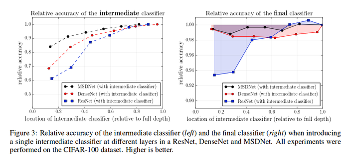
Figure 3 depicts relative accuracies of the intermediate classifiers and shows that the accuracy of a classifier is highly correlated with its position in the network. It is easy to see, specifically with the case of ResNet, that the classifiers improve in a staircase pattern. All of the experiments were performed on Cifar-100 dataset and it can be seen that the intermediate classifiers perform worst than the final classifiers, thus highlighting the problem with the lack of coarse level features early on.
To address this issue, MSDNets proposes an architecture in which uses multi scaled feature maps. The feature maps at a particular layer and scale are computed by concatenating results from up to two convolutions: a standard convolution is first applied to same-scale features from the previous layer to pass on high-resolution information that subsequent layers can use to construct better coarse features, and if possible, a strided convolution is also applied on the finer-scale feature map from the previous layer to produce coarser features amenable to classification. The network is quickly formed to contain a set number of scales ranging from fine to coarse. These scales are propagated throughout, so that for the length of the network there are always coarse level features for classification and fine features for learning more difficult representations.
Training of Early Classifiers Interferes with Later Classifiers
When training a network containing intermediate classifiers, the training of early classifiers will cause the early layers to focus on features for that classifier. These learned features may not be as useful to the later classifiers and degrade their accuracy.
MSDNets use dense connectivity to avoid this issue. By concatenating all prior layers to learn future layers, the gradient propagation is spread throughout the available features. This allows later layers to not be reliant on any single prior, providing opportunities to learn new features that priors have ignored.
Architecture

The architecture of MSDNet is a structure of convolutions with a set number of layers and a set number of scales. Layers allow the network to build on the previous information to generate more accurate predictions, while the scales allow the network to maintain coarse level features throughout.
The first layer is a special, mini-CNN-network, that quickly fills all required scales with features. The following layers are generated through the convolutions of the previous layers and scales.
Each output at a given s scale is given by the convolution of all prior outputs of the same scale, and the strided-convolution of all prior outputs from the previous scale.
The classifiers consists of two convolutional layers, an average pooling layer and a linear layer and are run on the concatenation of all of the coarsest outputs from the preceding layers.
Loss Function
The loss is calculated as a weighted sum of each classifier's logistic loss:
[math]\displaystyle{ \frac{1}{|\mathcal{D}|} \sum_{x,y \in \mathcal{D}} \sum_{k}w_k L(f_k) }[/math]
Here [math]\displaystyle{ w_i }[/math] represents the weights and [math]\displaystyle{ L(f_k) }[/math] represents the logistic loss of each classifier. The weighted loss is taken as an average over a set of training samples. The weights can be determined from a budget of computational power, but results also show that setting all to 1 is also acceptable.
Computational Limit Inclusion
When running in a budgeted batch scenario, the network attempts to provide the best overall accuracy. To do this with a set limit on computational resources, it works to use less of the budget on easy detections in order to allow more time to be spent on hard ones. In order to facilitate this, the classifiers are designed to exit when the confidence of the classification exceeds a preset threshold. To determine the threshold for each classifier, [math]\displaystyle{ |D_{test}|\sum_{k}(q_k C_k) \leq B }[/math] must be true. Where [math]\displaystyle{ |D_{test}| }[/math] is the total number of test samples, [math]\displaystyle{ C_k }[/math] is the computational requirement to get an output from the [math]\displaystyle{ k }[/math]th classifier, and [math]\displaystyle{ q_k }[/math] is the probability that a sample exits at the [math]\displaystyle{ k }[/math]th classifier. Assuming that all classifiers have the same base probability, [math]\displaystyle{ q }[/math], then [math]\displaystyle{ q_k }[/math] can be used to find the threshold.
Network Reduction and Lazy Evaluation
There are two ways to reduce the computational needs of MSDNets:
- Reduce the size of the network by splitting it into [math]\displaystyle{ S }[/math] blocks along the depth dimension and keeping the [math]\displaystyle{ (S-i+1) }[/math] scales in the [math]\displaystyle{ i^{\text{th}} }[/math] block.Whenever a scale is removed, a transition layer merges the concatenated features using 1x1 convolution and feeds the fine grained features to coarser scales.
- Remove unnecessary computations: Group the computation in "diagonal blocks"; this propagates the example along paths that are required for the evaluation of the next classifier.
The strategy of minimizing unnecessary computations when the computational budget is over is known as the lazy evaluation.
Experiments
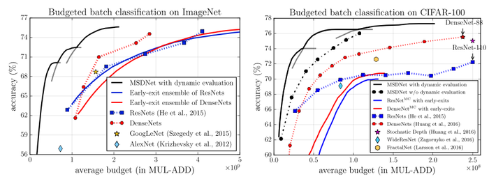
When evaluating on CIFAR-10 and CIFAR-100 ensembles and multi-classifier versions of ResNets and DenseNets, as well as FractalNet are used to compare with MSDNet.
When evaluating on ImageNet ensembles and individual versions of ResNets and DenseNets are compared with MSDNets.
Anytime Prediction
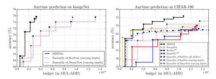
In anytime prediction MSDNets are shown to have highly accurate with very little budget, and continue to remain above the alternate methods as the budget increases. The authors attributed this to the fact that MSDNets are able to produce low-resolution feature maps well-suited for classification after just a few layers, in contrast to the high-resolution feature maps in early layers of ResNets or DenseNets. Ensemble networks need to repeat computations of similar low-level features repeatedly when new models need to be evaluated, so their accuracy results do not increase as fast when computational budget increases.
Budget Batch
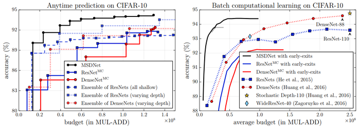
For budget batch 3 MSDNets are designed with classifiers set-up for varying ranges of budget constraints. On both dataset options the MSDNets exceed all alternate methods with a fraction of the budget required.
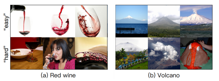
The following figure shows examples of what was deemed "easy" and "hard" examples by the network. The top row contains images of either red wine or volcanos that were easily classified, thus exiting the network early and reducing required computations. The bottom row contains examples of "hard" images that were incorrectly classified by the first classifier but were correctly classified by the last layer.
Ablation study
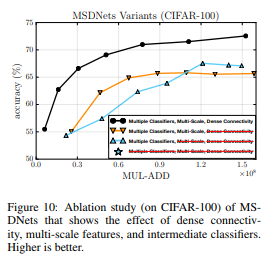
Additional experiments were performed to shed light on multi-scale feature maps, dense connectivity, and intermediate classifiers. This experiment started with an MSDNet with six intermediate classifiers and each of these components were removed, one at a time. To make our comparisons fair, the computational costs of the full networks were kept similar by adapting the network width. After removing all the three components, a VGG-like convolutional network is obtained. The classification accuracy of all classifiers is shown in the image below.
Critique
The problem formulation and scenario evaluation were very well formulated, and according to independent reviews, the results were reproducible. Where the paper could improve is on explaining how to implement the threshold; it isn't very well explained how the use of the validation set can be used to set the threshold value.
Implementation
The following repository provides the source code for the paper, written by the authors: https://github.com/gaohuang/MSDNet
Sources
- Huang, G., Chen, D., Li, T., Wu, F., Maaten, L., & Weinberger, K. Q. (n.d.). Multi-Scale Dense Networks for Resource Efficient Image Classification. ICLR 2018. doi:1703.09844
- Huang, G. (n.d.). Gaohuang/MSDNet. Retrieved March 25, 2018, from https://github.com/gaohuang/MSDNet
- LeCun, Yann, John S. Denker, and Sara A. Solla. "Optimal brain damage." Advances in neural information processing systems. 1990.
- Hassibi, Babak, David G. Stork, and Gregory J. Wolff. "Optimal brain surgeon and general network pruning." Neural Networks, 1993., IEEE International Conference on. IEEE, 1993.
- Li, Hao, et al. "Pruning filters for efficient convnets." arXiv preprint arXiv:1608.08710 (2016).
- Hubara, Itay, et al. "Binarized neural networks." Advances in neural information processing systems. 2016.
- Rastegari, Mohammad, et al. "Xnor-net: Imagenet classification using binary convolutional neural networks." European Conference on Computer Vision. Springer, Cham, 2016.
- Cristian Bucilua, Rich Caruana, and Alexandru Niculescu-Mizil. Model compression. In ACM SIGKDD, pp. 535–541. ACM, 2006.
- Geoffrey Hinton, Oriol Vinyals, and Jeff Dean. Distilling the knowledge in a neural network. In NIPS Deep Learning Workshop, 2014.
- Teerapittayanon, Surat, Bradley McDanel, and H. T. Kung. "Branchynet: Fast inference via early exiting from deep neural networks." Pattern Recognition (ICPR), 2016 23rd International Conference on. IEEE, 2016.
