One pixel attack for fooling deep neural networks
Presented by
1. Ziheng Chu
2. Minghao Lu
3. Qi Mai
4. Qici Tan
Introduction
Neural network first caught people’s attention during the 2012 imageNet contest. A solution using neural network achieve 85% accuracy, a large improvement from the previous 75% record. In the following year, NN were able to achieve 89% accuracy. In a short amount time, the ML community went from no-one using neural networks to everyone using the neural network. Today we have 97% accuracy in using deep neural network (DNN) on the imageNet dataset. So the problem of image classification using artificial intelligence is nearly a solved problem. However, there is one huge catch(Carlini.N,2017).
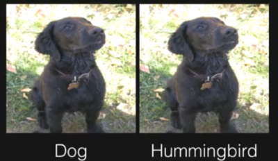
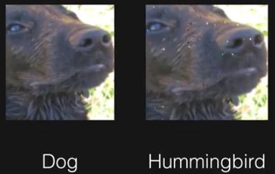
The catch is that the DNN can be quite vulnerable to intentional attacks. Here is an example, with a light modification, an image of a dog can be classified as a hummingbird. Research studies by Google Brian, which is a deep learning artificial intelligence research team, showed that any machine learning classifier can be tricked to give wrong predictions. The action of designing an input in a specific way to get the wrong result from the model is called an adversarial attack (Roman Trusov,2017). An adversarial image is created by adding a tiny amount of perturbation, which is not so imperceptible to human eyes as shown in Figure 1. After zooming into Figure 1, as shown in Figure 2, a small amount of perturbation led to misclassify a dog as a hummingbird.
How is it possible? DNN models consist of transformation. Most of those transformations are sometimes very sensitive to a small change. Think of the DNN as a set of high-dimensional decision boundary. When an input is not perfect, if the decision boundary is too simple and linear, mostly it leads to misclassify.
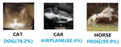
Harnessing this sensitivity is a way to better understand and produce more robust algorithm for AI security. This paper aims to demonstrate the vulnerability of DNN by presenting some extreme scenarios - one pixel attack. As shown in Figure3, even when only one pixel was perturbed, the classification is fooled for each image. Although, there is no profound defence to the attack currently, the investigation of one-pixel attack may shield lights on the behaviour of DNN and help develop defence techniques. Ultimately, it leads to the discussion of the security implications to future solution.
This paper proposes one-pixel attack in a scenario where the only information available is the probability labels. Comparing to previous work, this proposal showed its effectiveness of successful attack rate up to 73%, its simplicity of semi-black-box which only required probability label no need inner information, and its flexibility in attacking more models, especially the networks that are not differentiable and the gradient calculation is difficult.
With the intension of creating an adversarial attack for better understanding the security of DNN, one pixel attack should be considered. Two main reasons: 1) a new way of exploring the high dimensional DNN by using fewer and lower dimensional slices. It is different from previous work, where perturbation was done by adding small value to each pixel. 2) a measure of perceptiveness to demonstrate the severity of one-pixel attack as comparing to a few pixel examples.
Related works
The sensitivity to well-turned artificial perturbation were investigated in various related work.
1. First perturbation was crafted by several gradient-based algorithms using back- propagation for obtaining gradient information. (C. Szegedy et al. )[1]
2. Fast gradient sign algorithm for calculating effective perturbation It was with the hypotheses of the linearity and high-dimensions of inputs were the main reason of vulnerability. (I.J.Goodfellow et al.) [2]
3. Greedy perturbation searching method by assuming the linearity of DNN decision boundary (S.M Moosavi-Dezfooli et al.) Jacobian matrix to build “Adversarial Saliency Map” which indicates the effectiveness of conducting a fixed length perturbation through the direction of each axis (N. Papernot et al. )[3][4][5]
4. The images can hardly be recognized by human eyes but nevertheless classified by the network with high confi- dence. (A. Nguyen et al. )[6]
5. Several black-box attacks that require no internal knowledge about the target systems such as gradients, have also been proposed. only utilized it as a starting point to derive a further semi black-box attack which needs to modify more pixels (N. Narodytska et al)[7][8][9]
6. Both natural and random images are found to be vulnerable to adversarial perturbation. Assuming these images are evenly distributed, it suggests that most data points in the input space are gathered near to the boundaries. ( A. Fawzi, S. M. Moosavi Dezfooli, and P. Frossard.)[10]
7. A curvature analysis region along most directions around natural images are flat with only few directions where the space is curved and the images are sensitive to perturbation. (A. Fawzi et al.)[11]
8. Universal perturbations (i.e. a perturbation that when added to any natural image can generate adversarial samples with high effectiveness) were shown possible and to achieve a high effectiveness when compared to random perturbation. This indicates that the diversity of boundaries might be low while the boundaries’ shapes near different data points are similar (S. M. Moosavi Dezfooli, A. Fawzi, O. Fawzi, and P. Frossard.)[12]
Methodology
Problem Description
We can formalize the generation of adversarial images as an constrained optimization problem. We are given a classifier F and a targeted adversarial class adv. Let x be the vectorized form of an image. Let F_adv(x) represent the probability assigned to the targeted class adv for vector x by the given classifier. Let e(x) represent an additive adversarial perturbation vector for image x. This vector is to be added to the image vector x in order to fool the classifier into assigning a high probability for the given adversarial class. The goal of the targeted attack adversary is therefor to find the perturbation vector with constrained size(norm) that maximizes the probability assigned to the targeted class by the classifier. Formally

For few-pixel attack, the problem statement is changed slightly. We constrain on the number of non-zero elements of the perturbation vector instead of the norm of the vector.

For the usual adversarial case, we can shift x in all dimensions, but the strength(norm) of the shift is bounded by L. For our one-pixel attack case, we are using the second equation with d=1. x is only allowed to be perturbed along a single axis, so the degree of freedom of the shift is greatly reduces. However, the shift in the one axis can be of arbitrary strength.
Differential Evolution
Differential evolution(DE) is a stochastic, population based optimization algorithm belonging to the class of evolutionary algorithms(EA). DE does not make assumptions of the underlying fitness landscape. It does not require an explicit form of the fitness function nor the associated gradient information, which makes it suitable for our task. Like other evolutionary algorithms, DE starts with a population of feasible solutions, and then loops between expanding the population by performing mutation and recombination, and reducing the population by performing fitness based selection. When certain convergence criteria is met, the most fit solution from the population is chosen as the final result.

DE makes the explicit assumption that solutions can be encoded into vectors. For DE, in the selection process, the population is in a way "segmented" into families( offspring and parents ), and the most optimal from each family is chosen. This segmentation allows DE to keep more diversity in each iteration than other EAs and makes it more suitable for complex multi-modal optimization problems.
Algorithm
For our problem, perturbation are encoded into five element tuples, representing the x-y coordinates and the RBG value of the perturbation. Each perturbation modifies exactly one pixel. Each candidate solution is a vector of perturbations. The initial iteration has 400 candidate solutions, and each iteration produces 400 more candidate solutions. Child candidate solutions are produced by the formula

where x is an element of the candidate solution. r1, r2, r3 are random numbers and represent choosing random partners for mutation and recombination. F is the differential weight set to be 0.5. g is the current generation. Each child solution competes with its parent, and the more fit solution is kept for the next iteration. The maximum number of iteration is set to 100.
The initial population is randomly generated using uniform distribution for choosing pixel to modify, and gaussian distribution with mean 128 and standard deviation 127 to choose each colour's offset. The fitness function is simply the output probability of the given classifier on the perturbed image for the targeted adversarial class.
Evaluation and Results
Measurement Metrics and Datasets
The authors used 4 measurement metrics to evaluate the effectiveness of the proposed attacks.
- Success Rate
Non-targeted attack: the percentage of adversarial images were successfully classified to any possible classes other than the true one.
- [math]\displaystyle{ \textrm{success rate }=\displaystyle\sum_{k=1}^N I(\textrm{Network}(\textrm{Attack}(\textrm{Image}_k))\neq \textrm{TrueClass}_k) }[/math]
Targeted attack: the probability of successfully classifying a perturbed image to a targeted class. - [math]\displaystyle{ \textrm{success rate }=\displaystyle\sum_{k=1}^N I(\textrm{Network}(\textrm{TargetedAttack}(\textrm{Image}_k))= \textrm{TrueClass}_k) }[/math]
- Adversarial Probability Labels (Confidence)
The ratio of sum of probability level of the target class for each successful perturbation and the total number of successful attacks. This gives the mean confidence of the successful attacks on the target classification system. - Number of Target Classes
The number of images after perturbations cannot be classified to any other classes. - Number of Original-Target Class Pairs
The number of times of each pair being attacked.
Evaluation setups on CIFAR-10 test dataset:
Three types of networks played as defense systems: All Convolutional Networks (AllConv), Network in Network (NiN) and VGG16 network. (Figure 1)
The authors randomly sampled 500 images, with resolution 32x32x3, from the dataset to perform one-pixel attacks and generated 500 samples with 3 and 5 pixel-modification respectively to conduct three-pixel and five-pixel attacks. The effectiveness of one-pixel attack was evaluated on all three introduced networks and the performance comparison, using success rate, was performed as the following: 1-pixel attack and 3-pixel attack on AllConv and 5-pixel attack on NiN.
Both targeted attacks and non-targeted attacks were considered but only targeted attacks were conducted since the performance of non-targeted attack results could be obtained from the result of targeted attacks by applying a fitness function to increase the probability level of the target class.
Evaluation setups on ImageNet validation dataset (ILSVRC 2012):
BVLC AlexNet played as defense system. (Figure 1)
600 sample images were randomly sampled from the dataset. Due to the relatively high resolution of the images (224x224x3), only one-pixel attacked was carried out aiming to verify if extremely small pixel modification in a relatively large image can alternate the classification result.
Since the number of classes in this dataset is way larger than the one of CIFAR-10, the authors only launched non-targeted attacks and applied a fitness function to decrease the probability level of the true class.
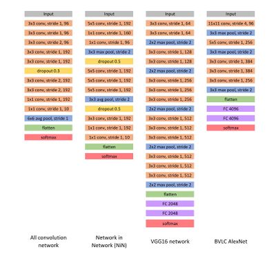
Results
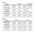
On CIFAR-10, the proposed one-pixel attack succeeded (Table 1) in general and success rate and confidence increased by a significant amount when more pixels were modified (Table 2). Moreover, with one-pixel modification, each image can be perturbed to 2~4 classes in all 3 defense systems, i.e. AllConv, NiN and VGG16 (Figure 2); in particular, VGG16 is slightly more robust than the other two. Generally, all these three networks are vulnerable to one-pixel attack. When more pixels were allowed modifications, a significant number of images were successfully perturbed to up to 8 classes (Figure 3).
On ImageNet, one-pixel attack performed well regarding to relatively large images (Table 1). The low confidence 5.53% is due to the large number of classes and the main efforts in decreasing the probability level of the true class.
By comparing the non-targeted attack effectiveness between the proposed method and two previous works, single dimensional perturbation vector is enough to delivery the corresponding adversarial images for most of the samples (Figure 4).
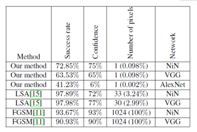
Also, it is easy to craft adversarial images for certain original-target class pairs, especially in the case of one-pixel attack, as the data points of these classes share the vulnerable target directions. However, by increasing the dimensions of perturbations (e.g. from 1 to 3 and 5), most original classes are equally robust and have similar number of adversarial images (Figure 5).
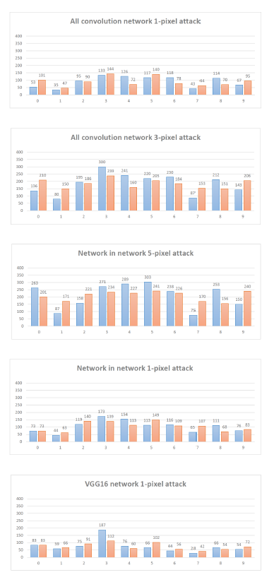
For special case (e.g. the ship when attacking NiN networks, class 8), it is relatively simple to craft adversarial samples from it but difficult to craft adversarial samples to it. Reason behind it is that, the boundary shape of the class is long and thin with natural images close to the border.
In order to evaluate the time cost of conducting one-pixel attack for the four types of networks, the writer uses 2 metrics:
1. AvgEvaluation: the average number of evaluations to produce adversarial images
2. AvgDistortion: the required average distortion in one-colour channel of a single pixel to produce adversarial images
The result is summarized in Figure 6:

Discussion and Future Work
This paper illustrates the possibility of finding point boundaries where class labels changes by moving data points along few dimensions and analyzing the frequency of changes in class labels quantitatively; it also proves that a single pixel change is powerful enough to perturb a considerable portion of images and the one-pixel attack can further work on different network structures or image sizes. Given the time constraints, the conducted experiments used a low number of DE iterations with a relatively small set of initial candidate solutions; by increasing the number of DE iterations or the initial candidate solutions, the perturbation success rate can be further improved.
For the future work, it is suggested to use the proposed algorithms and natural image samples for further development of advanced models and better artificial adversarial samples.
Critique
- When the authors launched 1, 3 and 5-pixel attacks, they did it on different target networks, i.e. 1 and 3-pixel attacks on AllConv and 5-pixel attack on NiN, then compared the corresponding success rates. Such a comparison is not rigorous as different networks might lead to varied classification results. Although we understand that the authors wanted to show the best attack results among those networks, we think all three attacks should be conducted on the same defense systems respectively and consequently we can see the performance of each attack on each target network. The conclusion from these results would be more convincing.
- Regarding to ImageNet, only AlexNet was used to attack but AllConv, NiN and VGG16. The papers in which AllConv and VGG16 were introduced have good experiment results on ImageNet. Attack experiments towards these networks should be considered to show the effectiveness of one-pixel attack.
Reference
Carlini.N,2017 https://www.youtube.com/watch?v=yIXNL88JBWQ
Jiawei Su, Danilo Vasconcellos Vargas, Sakurai Kouichi, 2017 https://arxiv.org/pdf/1710.08864.pdf
Roman Trusov,2017 https://blog.xix.ai/how-adversarial-attacks-work-87495b81da2d
