Neural Audio Synthesis of Musical Notes with WaveNet autoencoders
Introduction
The authors of this paper have pointed out that the method in which most notes are created are hand-designed instruments modifying pitch, velocity and filter parameters to produce the required tone, timbre and dynamics of a sound. The authors suggest that this may be a problem and thus suggest a data-driven approach to audio synthesis. They demonstrate how to generate new types of expressive and realistic instrument sounds using a neural network model instead of using specific arrangements of oscillators or algorithms for sample playback. The model is capable of learning semantically meaningful hidden representations which can be used as control signals for manipulating tone, timbre, and dynamics during playback. To train such a data expensive model the authors highlight the need for a large dataset much like imagenet for music. The motivation for this work stems from recent advances in autoregressive models like WaveNet [5] and SampleRNN [6]. These models are effective at modeling short and medium scale (~500ms) signals, but rely on external conditioning for large-term dependencies; the proposed model removes the need for external conditioning.
Contributions
To solve the problem highlighted above the authors propose two main contributions of their paper:
- Wavenet-style autoencoder that learn to encode temural data over a long term audio structures without requiring external conditioning
- NSynth: a large dataset of musical notes inspired by the emerging of large image datasets
Models
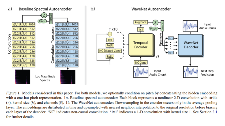
WaveNet Autoencoder
While the proposed autoencoder structure is very similar to that of WaveNet the authors argue that the algorithm is novel in two ways:
- It is able to attain consistent long-term structure without any external conditioning
- Creating meaningful embedding which can be interpolated between
The authors accomplish this by passing the raw audio throw the encoder to produce an embedding [math]\displaystyle{ Z = f(x) }[/math], next the input is shifted and feed into the decoder which reproduces the input. The resulting probability distribution:
\begin{align} p(x) = \prod_{i=1}^N\{x_i | x_1, … , x_N-1, f(x) \} \end{align}
A detailed block diagram of the modified WaveNet structure can be seen in figure 1b. This diagram demonstrates the encoder as a 30 layer network in each each node is a ReLU nonlinearity followed by a non-causal dilated convolution. Dilated convolution (aka convolutions with holes) is a type of convolution in which the filter skips input values with a certain step (step size of 1 is equivalent to the standard convolution), effectively allowing the network to operate at a coarser scale compared to traditional convolutional layers and have very large receptive fields. The resulting convolution is 128 channels all feed into another ReLU nonlinearity which is feed into another 1x1 convolution before getting down sampled with average pooling to produce a 16 dimension [math]\displaystyle{ Z }[/math] distribution. Each [math]\displaystyle{ Z }[/math] encoding is for a specific temporal resolution which the authors of the paper tuned to 32ms. This means that there are 125, 16 dimension [math]\displaystyle{ Z }[/math] encodings for each 4 second note present in the NSynth database (1984 embeddings). Before the [math]\displaystyle{ Z }[/math] embedding enters the decoder it is first upsampled to the original audio rate using nearest neighbor interpolation. The embedding then passes through the decoder to recreate the original audio note. The input audio data is first quantized using 8-bit mu-law encoding into 256 possible values, and the output prediction is the softmax over the possible values.
Baseline: Spectral Autoencoder
Being unable to find an alternative fully deep model which the authors could use to compare to there proposed WaveNet autoencoder to, the authors just made a strong baseline. The baseline algorithm that the authors developed is a spectral autoencoder. The block diagram of its architecture can be seen in figure 1a. The baseline network is 10 layer deep. Each layer has a 4x4 kernels with 2x2 strides followed by a leaky-ReLU (0.1) and batch normalization. The final hidden vector(Z) was set to 1984 to exactly match the hidden vector of the WaveNet autoencoder.
The authors attempted to train the baseline on multiple input: raw waveforms, FFT, and log magnitude of spectrum finding the latter to be best correlated with perceptual distortion. The authors also explored several representations of phase, finding that estimating magnitude and using established iterative techniques to reconstruct phase to be most effective. (The technique to reconstruct the phase from the magnitude comes from (Griffin and Lim 1984). It can be summarized as follows. In each iteration, generate a Fourier signal z by taking the Short Time Fourier transform of the current estimate of the complete time-domain signal, and replacing its magnitude component with the known true magnitude. Then find the time-domain signal whose Short Time Fourier transform is closest to z in the least-squares sense. This is the estimate of the complete signal for the next iteration. ) A final heuristic that was used by the authors to increase the accuracy of the baseline was weighting the mean square error (MSE) loss starting at 10 for 0 HZ and decreasing linearly to 1 at 4000 Hz and above. This is valid as the fundamental frequency of most instrument are found at lower frequencies.
Training
Both the modified WaveNet and the baseline autoencoder used stochastic gradient descent with an Adam optimizer. The authors trained the baseline autoencoder model asynchronously for 1800000 epocs with a batch size of 8 with a learning rate of 1e-4. Where as the WaveNet modules were trained synchronously for 250000 epocs with a batch size of 32 with a decaying learning rate ranging from 2e-4 to 6e-6.
The NSynth Dataset
To evaluate the WaveNet autoencoder model, the authors' wanted an audio dataset that let them explore the learned embeddings. Musical notes are an ideal setting for this study. Prior to this paper, the existing music datasets included the RWC music database (Goto et al., 2003) and the dataset from Romani Picas et al. However, the authors wanted to develop a larger dataset.
The NSynth dataset has 306 043 unique musical notes (each have a unique pitch, timbre, envelope) all 4 seconds in length sampled at 16,000 Hz. The data set consists of 1006 different instruments playing on average of 65.4 different pitches across on average 4.75 different velocities. Average pitches and velocities are used as not all instruments, can reach all 88 MIDI frequencies, or the 5 velocities desired by the authors. The dataset has the following split: training set with 289,205 notes, validation set with 12,678 notes, and test set with 4,096 notes.
Along with each note the authors also included the following annotations:
- Source - The way each sound was produced. There were 3 classes ‘acoustic’, ‘electronic’ and ‘synthetic’
- Family - The family class of instruments that produced each note. There is 11 classes which include: {‘bass’, ‘brass’, ‘vocal’ ext.}
- Qualities - Sonic qualities about each note
The full dataset is publicly available here: https://magenta.tensorflow.org/datasets/nsynth.
Evaluation
To fully analyze all aspects of WaveNet the authors proposed three evaluations:
- Reconstruction - Both Quantitative and Qualitative analysis were considered
- Interpolation in Timbre and Dynamics
- Entanglement of Pitch and Timbre
Sound is historically very difficult to quantify from a picture representation as it requires training and expertise to analyze. Even with expertise it can be difficult to complete a full analyses as two very different sound can look quite similar in the respective pictorial representation. This is why the authors recommend all readers to listen to the created notes which can be sound here: https://magenta.tensorflow.org/nsynth.
However, even when taking this under consideration the authors do pictorially demonstrate differences in the two proposed algorithms along with the original note, as it is hard to publish a paper with sound included. To demonstrate the pictorial difference the authors demonstrate each note using constant-q transform (CQT) which is able to capture the dynamics of timbre along with representing the frequencies of the sound.
Reconstruction
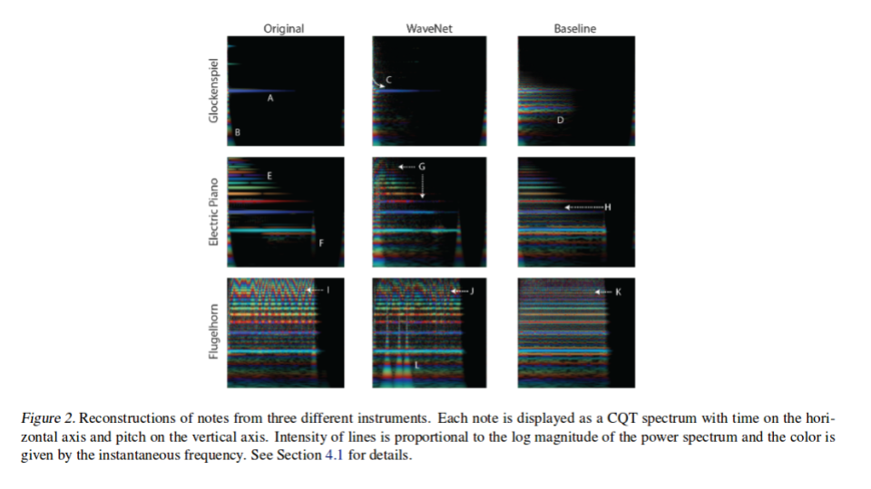
Qualitative Comparison
In the Glockenspiel the WaveNet autoencoder is able to reproduce the magnitude, phase of the fundamental frequency (A and C in figure 2), and the attack (B in figure 2) of the instrument; Whereas the Baseline autoencoder introduces non existing harmonics (D in figure 2). The flugelhorn on the other hand, presents the starkest difference between the WaveNet and baseline autoencoders. The WaveNet while not perfect is able to reproduce the verbarto (I and J in figure 2) across multiple frequencies, which results in a natural sounding note. The baseline not only fails to do this but also adds extra noise (K in figure 2). The authors do add that the WaveNet produces some strikes (L in figure 2) however they argue that they are inaudible.
Mu-law encoding was used in the original WaveNet paper to make the problem "more tractable" compared to raw 16-bit integer values. In that paper, they note that "especially for speech, this non-linear quantization produces a significantly better reconstruction" compared to a linear scheme. This might be expected considering that the mu-law companding transformation was designed to encode speech. In this application though, using this encoding creates perceptible distortion that sounds similar to clipping.
Quantitative Comparison
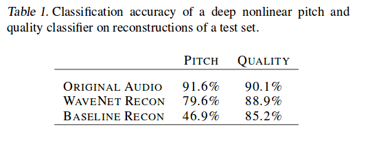
For a quantitative comparison the authors trained a separate multi-task classifier to classify a note using given pitch or quality of a note. The results of both the Baseline and the WaveNet where then inputted and attempted to be classified. As seen in table 1 WaveNet significantly outperformed the Baseline in both metrics posting a ~70% increase when only considering pitch.
Interpolation in Timbre and Dynamics
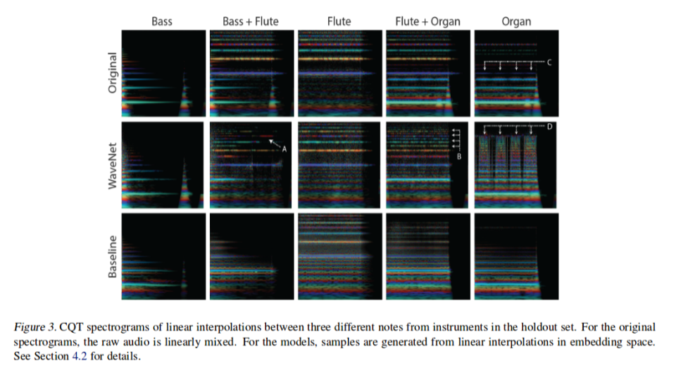
For this evaluation the authors reconstructed from linear interpolations in Z space among different instruments and compared these to superimposed position of the original two instruments. Not surprisingly the model fuse aspects of both instruments during the recreation. The authors claim however, that WaveNet produces much more realistic sounding results. To support their claim the authors the authors point to WaveNet ability to create dynamic mixing of overtone in time, even jumping to higher harmonics (A in figure 3), capturing the timbre and dynamics of both the bass and flute. This can be once again seen in (B in figure 3) where Wavenet adds additional harmonics as well as a sub-harmonics to the original flute note.
Entanglement of Pitch and Timbre
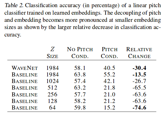
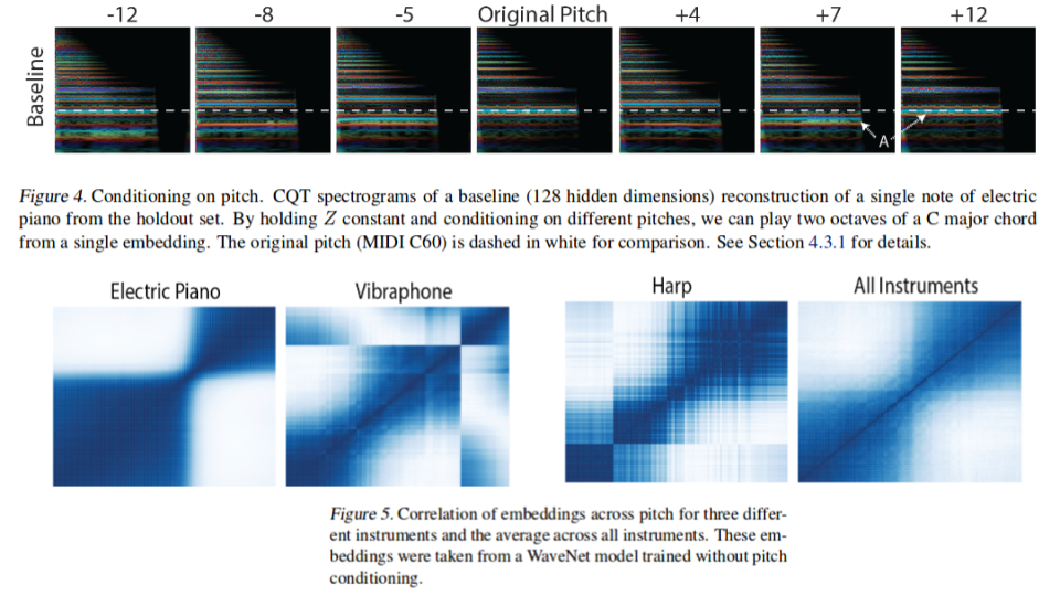
To study the entanglement between pitch and Z space the authors constructed a classifier which was expected to drop in accuracy if the representation of pitch and timbre is disentangled as it relies heavily on the pitch information. This is clearly demonstrated by the first two rows of table 2 where WaveNet relies more strongly on pitch then the baseline algorithm. The authors provide a more qualitative demonstrating in figure 4. They demonstrate a situation in which a classifier may be confused; a note with pitch of +12 is almost exactly the same as the original apart from an emergence of sub-harmonics.
Further insight can be gained on the relationship between pitch and timbre by studying the trend amongst the network embeddings among the pitches for specific instruments. This is depicted in figure 5 for several instruments across their entire 88 note range at 127 velocity. It can be noted from the figure that the instruments have unique separation of two or more registers over which the embeddings of notes with different pitches are similar. This is expected since instrumental dynamics and timbre varies dramatically over the range of the instrument.
Future Directions
One significant area which the authors claim great improvement is needed is the large memory constraints required by there algorithm. Due to the large memory requirement the current WaveNet must rely on down sampling thus being unable to fully capture the global context. They claim that research using different input representations (instead of mu-law) to minimize distortion is ongoing.
Open Source Code
Google has released all code related to this paper at the following open source repository: https://github.com/tensorflow/magenta/tree/master/magenta/models/nsynth
References
- Engel, J., Resnick, C., Roberts, A., Dieleman, S., Norouzi, M., Eck, D. & Simonyan, K.. (2017). Neural Audio Synthesis of Musical Notes with WaveNet Autoencoders. Proceedings of the 34th International Conference on Machine Learning, in PMLR 70:1068-1077
- Griffin, Daniel, and Jae Lim. "Signal estimation from modified short-time Fourier transform." IEEE Transactions on Acoustics, Speech, and Signal Processing 32.2 (1984): 236-243.
- NSynth: Neural Audio Synthesis. (2017, April 06). Retrieved March 19, 2018, from https://magenta.tensorflow.org/nsynth
- The NSynth Dataset. (2017, April 05). Retrieved March 19, 2018, from https://magenta.tensorflow.org/datasets/nsynth
- Oord, Aaron van den, Nal Kalchbrenner, and Koray Kavukcuoglu. "Pixel recurrent neural networks." arXiv preprint arXiv:1601.06759 (2016).
- Mehri, Soroush, et al. "SampleRNN: An unconditional end-to-end neural audio generation model." arXiv preprint arXiv:1612.07837 (2016).