stat946w18/Implicit Causal Models for Genome-wide Association Studies
Introduction and Motivation
There is currently much progress in probabilistic models which could lead to the development of rich generative models. The models have been applied with neural networks, implicit densities, and with scalable algorithms to very large data for their Bayesian inference. However, most of the models are focused on capturing statistical relationships rather than causal relationships. Causal models give us a sense of how manipulating the generative process could change the final results.
Genome-wide association studies (GWAS) are examples of causal relationships. Specifically, GWAS is about figuring out how genetic factors cause disease among humans. Here the genetic factors we are referring to are single nucleotide polymorphisms (SNPs), and getting a particular disease is treated as a trait, i.e., the outcome. In order to know about the reason of developing a disease and to cure it, the causation between SNPs and diseases is investigated: first, predict which one or more SNPs cause the disease; second, target the selected SNPs to cure the disease.
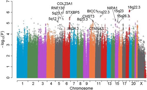
The figure below depicts an example Manhattan plot for a GWAS. Each dot represents an SNP. The x-axis is the chromosome location, and the y-axis is the negative log of the association p-value between the SNP and the disease, so points with the largest values represent strongly associated risk loci.

This paper dealt with two questions. The first one is how to build rich causal models with specific needs by GWAS. In general, probabilistic causal models involve a function [math]\displaystyle{ f }[/math] and a noise [math]\displaystyle{ n }[/math]. For working simplicity, we usually assume [math]\displaystyle{ f }[/math] as a linear model with Gaussian noise. However, it has been proven that in GWAS, it is necessary to accommodate non-linearity and interactions between multiple genes into the models.
The second accomplishment of this paper is that it addressed the problem caused by latent confounders. Latent confounders are issues when we apply the causal models since we cannot observe them nor know the underlying structure. In this paper, they developed implicit causal models which can adjust for confounders.
There has been an increasing number of works on causal models which focus on causal discovery and typically have strong assumptions such as Gaussian processes on noise variable or nonlinearities for the main function.
Implicit Causal Models
Implicit causal models are an extension of probabilistic causal models. Probabilistic causal models will be introduced first.
Probabilistic Causal Models
Probabilistic causal models have two parts: deterministic functions of noise and other variables. Consider a global variable [math]\displaystyle{ \beta }[/math] and noise [math]\displaystyle{ \epsilon }[/math], where

Each [math]\displaystyle{ \beta }[/math] and [math]\displaystyle{ x }[/math] is a function of noise; [math]\displaystyle{ y }[/math] is a function of noise and [math]\displaystyle{ x }[/math],

The target is the causal mechanism [math]\displaystyle{ f_y }[/math] so that the causal effect [math]\displaystyle{ p(y|do(X=x),\beta) }[/math] can be calculated. [math]\displaystyle{ do(X=x) }[/math] means that we specify a value of [math]\displaystyle{ X }[/math] under the fixed structure [math]\displaystyle{ \beta }[/math]. By other paper’s work, it is assumed that [math]\displaystyle{ p(y|do(x),\beta) = p(y|x, \beta) }[/math].

An example of probabilistic causal models is additive noise model.

[math]\displaystyle{ f(.) }[/math] is usually a linear function or spline functions for nonlinearities. [math]\displaystyle{ \epsilon }[/math] is assumed to be standard normal, as well as [math]\displaystyle{ y }[/math]. Thus the posterior [math]\displaystyle{ p(\theta | x, y, \beta) }[/math] can be represented as

where [math]\displaystyle{ p(\theta) }[/math] is the prior which is known. Then, variational inference or MCMC can be applied to calculate the posterior distribution.
Implicit Causal Models
The difference between implicit causal models and probabilistic causal models is the noise variable. Instead of an additive noise term, implicit causal models directly take noise [math]\displaystyle{ \epsilon }[/math] into a neural network and output [math]\displaystyle{ x }[/math].
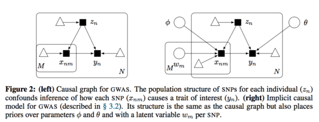
The causal diagram has changed to:

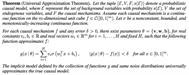
They used fully connected neural network with a fair amount of hidden units to approximate each causal mechanism. Below is the formal description:

Implicit Causal Models with Latent Confounders
Previously, they assumed the global structure is observed. Next, the unobserved scenario is being considered.
Causal Inference with a Latent Confounder
Same as before, the interest is the causal effect [math]\displaystyle{ p(y|do(x_m), x_{-m}) }[/math]. Here, the SNPs other than [math]\displaystyle{ x_m }[/math] is also under consideration. However, it is confounded by the unobserved confounder [math]\displaystyle{ z_n }[/math]. As a result, the standard inference method cannot be used in this case.
The paper proposed a new method which include the latent confounders. For each subject [math]\displaystyle{ n=1,…,N }[/math] and each SNP [math]\displaystyle{ m=1,…,M }[/math],

The mechanism for latent confounder [math]\displaystyle{ z_n }[/math] is assumed to be known. SNPs depend on the confounders and the trait depends on all the SNPs and the confounders as well.
The posterior of [math]\displaystyle{ \theta }[/math] is needed to be calculate in order to estimate the mechanism [math]\displaystyle{ g_y }[/math] as well as the causal effect [math]\displaystyle{ p(y|do(x_m), x_{-m}) }[/math], so that it can be explained how changes to each SNP [math]\displaystyle{ X_m }[/math] cause changes to the trait [math]\displaystyle{ Y }[/math].

Note that the latent structure [math]\displaystyle{ p(z|x, y) }[/math] is assumed known.
In general, causal inference with latent confounders can be dangerous: it uses the data twice, and thus it may bias the estimates of each arrow [math]\displaystyle{ X_m → Y }[/math]. Why is this justified? This is answered below:
Proposition 1. Assume the causal graph of Figure 2 (left) is correct and that the true distribution resides in some configuration of the parameters of the causal model (Figure 2 (right)). Then the posterior [math]\displaystyle{ p(θ | x, y) }[/math] provides a consistent estimator of the causal mechanism [math]\displaystyle{ f_y }[/math].
Proposition 1 rigorizes previous methods in the framework of probabilistic causal models. The intuition is that as more SNPs arrive (“M → ∞, N fixed”), the posterior concentrates at the true confounders [math]\displaystyle{ z_n }[/math], and thus we can estimate the causal mechanism given each data point’s confounder [math]\displaystyle{ z_n }[/math]. As more data points arrive (“N → ∞, M fixed”), we can estimate the causal mechanism given any confounder [math]\displaystyle{ z_n }[/math] as there is an infinity of them.
Implicit Causal Model with a Latent Confounder
This section is the algorithm and functions to implementing an implicit causal model for GWAS.
Generative Process of Confounders [math]\displaystyle{ z_n }[/math].
The distribution of confounders is set as standard normal. [math]\displaystyle{ z_n \in R^K }[/math] , where [math]\displaystyle{ K }[/math] is the dimension of [math]\displaystyle{ z_n }[/math] and [math]\displaystyle{ K }[/math] should make the latent space as close as possible to the true population structural.
Generative Process of SNPs [math]\displaystyle{ x_{nm} }[/math].
Given SNP is coded for,

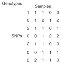
The authors defined a [math]\displaystyle{ Binomial(2,\pi_{nm}) }[/math] distribution on [math]\displaystyle{ x_{nm} }[/math]. And used logistic factor analysis to design the SNP matrix.

A SNP matrix looks like this:

Since logistic factor analysis makes strong assumptions, this paper suggests using a neural network to relax these assumptions,

This renders the outputs to be a full [math]\displaystyle{ N*M }[/math] matrix due the the variables [math]\displaystyle{ w_m }[/math], which act as principal component in PCA. Here, [math]\displaystyle{ \phi }[/math] has a standard normal prior distribution. The weights [math]\displaystyle{ w }[/math] and biases [math]\displaystyle{ \phi }[/math] are shared over the [math]\displaystyle{ m }[/math] SNPs and [math]\displaystyle{ n }[/math] individuals, which makes it possible to learn nonlinear interactions between [math]\displaystyle{ z_n }[/math] and [math]\displaystyle{ w_m }[/math].
Generative Process of Traits [math]\displaystyle{ y_n }[/math].
Previously, each trait is modeled by a linear regression,

This also has very strong assumptions on SNPs, interactions, and additive noise. It can also be replaced by a neural network which only outputs a scalar,

Likelihood-free Variational Inference
Calculating the posterior of [math]\displaystyle{ \theta }[/math] is the key of applying the implicit causal model with latent confounders.

could be reduces to

However, with implicit models, integrating over a nonlinear function could be suffered. The authors applied likelihood-free variational inference (LFVI). LFVI proposes a family of distribution over the latent variables. Here the variables [math]\displaystyle{ w_m }[/math] and [math]\displaystyle{ z_n }[/math] are all assumed to be Normal,

For LFVI applied to GWAS, the algorithm which similar to the EM algorithm has been used:

Empirical Study
The authors performed simulation on 100,000 SNPs, 940 to 5,000 individuals, and across 100 replications of 11 settings. Four methods were compared:
- implicit causal model (ICM);
- PCA with linear regression (PCA);
- a linear mixed model (LMM);
- logistic factor analysis with inverse regression (GCAT).
The feedforward neural networks for traits and SNPs are fully connected with two hidden layers using ReLU activation function, and batch normalization.
Simulation Study
Based on real genomic data, a true model is applied to generate the SNPs and traits for each configuration. There are four datasets used in this simulation study:
- HapMap [Balding-Nichols model]
- 1000 Genomes Project (TGP) [PCA]
- Human Genome Diversity project (HGDP) [PCA]
- HGDP [Pritchard-Stephens-Donelly model]
- A latent spatial position of individuals for population structure [spatial]
The table shows the prediction accuracy. The accuracy is calculated by the rate of the number of true positives divide the number of true positives plus false positives. True positives measure the proportion of positives that are correctly identified as such (e.g. the percentage of SNPs which are correctly identified as having the causal relation with the trait). In contrast, false positives state the SNPs has the causal relation with the trait when they don’t. The closer the rate to 1, the better the model is since false positives are considered as the wrong prediction.

The result represented above shows that the implicit causal model has the best performance among these four models in every situation. Especially, other models tend to do poorly on PSD and Spatial when [math]\displaystyle{ a }[/math] is small, but the ICM achieved a significantly high rate. The only comparable method to ICM is GCAT, when applying to simpler configurations.
Real-data Analysis
They also applied ICM to a real-world GWAS of Northern Finland Birth Cohorts which contain 324,160 SNPs and 5,027 individuals. Ten implicit causal models were fitted and the 2 neural networks both with two hidden layers were used for SNP and trait. The dimension of confounders ([math]\displaystyle{ K }[/math]) was set to be six, same as what was used in the paper by Song et al. for comparable models in Table 2.

The numbers in the above table are the number of significant loci for each of the 10 traits. The number for other methods, such as GCAT, LMM, PCA, and "uncorrected" (association tests without accounting for hidden relatedness of study samples) are obtained from other papers. By comparison, the ICM reached the level of the best previous model for each trait.
Conclusion
This paper introduced implicit causal models in order to account for nonlinear complex causal relationships, and applied the method to GWAS. It can not only capture important interactions between genes within an individual and among population level, but also can adjust for latent confounders by taking account of the latent variables into the model.
By the simulation study, the authors proved that the implicit causal model could beat other methods by 15-45.3% on a variety of datasets with variations on parameters.
The authors also believed this GWAS application is only a start of the usage of implicit causal models. It might also be used in physics or economics.
Critique
I think this paper is an interesting and novel work. The main contribution of this paper is to connect the statistical genetics and the machine learning methodology. The method is technically sound and does indeed generalize techniques currently used in statistical genetics.
The neural network used in this paper is a very simple feedforward 2 hidden-layer neural network, but the idea of where to use the neural network is crucial and might be significant in GWAS.
It has limitations as well. The empirical example in this paper is too easy, and far away from the realistic situation. Despite the simulation study showing some competing results, the Northern Finland Birth Cohort Data application did not demonstrate the advantage of using implicit causal model over the previous methods, such as GCAT or LMM.
Another limitation is about linkage disequilibrium as the authors stated as well. SNPs are not completely independent of each other; usually, they have correlations when the alleles at close locus. They did not consider this complex case, rather they only considered the simplest case where they assumed all the SNPs are independent.
Furthermore, one SNP maybe does not have enough power to explain the causal relationship. Recent papers indicate that causation to a trait may involve multiple SNPs. This could be a future work as well.
References
Tran D, Blei D M. Implicit Causal Models for Genome-wide Association Studies[J]. arXiv preprint arXiv:1710.10742, 2017.
Patrik O Hoyer, Dominik Janzing, Joris M Mooij, Jonas Peters, and Prof Bernhard Schölkopf. Non- linear causal discovery with additive noise models. In Neural Information Processing Systems, 2009.
Alkes L Price, Nick J Patterson, Robert M Plenge, Michael E Weinblatt, Nancy A Shadick, and David Reich. Principal components analysis corrects for stratification in genome-wide association studies. Nature Genetics, 38(8):904–909, 2006.
Minsun Song, Wei Hao, and John D Storey. Testing for genetic associations in arbitrarily structured populations. Nature, 47(5):550–554, 2015.
Dustin Tran, Rajesh Ranganath, and David M Blei. Hierarchical implicit models and likelihood-free variational inference. In Neural Information Processing Systems, 2017.