stat441w18/Image Question Answering using CNN with Dynamic Parameter Prediction
Image Question Answering using CNN with Dynamic Parameter Prediction
Presented by
Rosie Zou, Kye Wei, Glen Chalatov, Ameer Dharamshi
Introduction
Problem Setup
Historically, computer vision has been an incredibly challenging, yet equally important task for researchers. The ultimate goal of computer vision is to develop a system that can achieve a holistic understanding of an image to extract meaningful insights. After many years with limited progress towards this goal, the field had fallen out of the spotlight. However, the past decade has seen a resurgence of interest in computer vision research due to breakthroughs in deep learning and advancements in computational capabilities. Recent advances in the recognition capabilities of such systems has paved the way for further advances towards our ultimate objective.
Image question answering (Image Q&A) is the next stage. Image Q&A is the task of asking a system various questions about an image. This extends beyond simple recognition and requires detecting many objects within an image as well as finding some level of context in order to answer the question. The core challenge of Image Q&A is that the set of objects to detect and the level of understanding required is dependent on the question being asked. If the question was static, the model could be optimized based on the question. A broader Image Q&A model must be flexible in order to adapt to different questions.
From a model perspective, the question being posed must be incorporated into the model and processed at some point. Previous methods tend to extract image features from the image and descriptors from the question and present the intersection of these two sets as the answer. Previous models incorporate the question directly as an independent variable when determining the answer. This is written as: ![]()
Where ‘ahat’ is the best predicted answer, ‘omega’ is the set of all possible answers ‘a’, ‘I’ is the image, ‘q’ is the question, and ‘theta’ is the model parameter vector.
The authors of this paper propose using the question to set certain model parameters and thus use the question directly when extracting information from the picture. This is written as ![]()
Where ‘ahat’, ‘a’, ‘I’ are the same as above but ‘thetas’ is the vector of static parameters and ‘thetad(q)’ is the vector of dynamic parameters determined by the question.
This approach hopes to adapt the model to the specifics of the question. Intuitively, it is determining the answer based on the question instead of seeking the common features of both the question and the answer.
Previous and Related Works
As mentioned in the earlier section, one of the major goals in computer vision is to achieve holistic understanding. While relatively new interest in the computer vision community, Image Question Answering already has a growing number of researchers working on this problem. There has been many past and recent efforts on this front, for instance this non-exhaustive list of papers published between 2015 and 2016 (NIPS 2015 paper, ICCV 2015 paper, AAAI 2016 paper). One key commonality in these papers is that most, if not all, of the recognition problems are defined in a simple, controlled environment with a finite set of objectives. While the question-handling strategies differ from paper to paper, a general problem-solving strategy in these papers is to use CNNs for feature extraction from images prior to handling question sentences.
In contrast, there has been less efforts in solving various recognition problems simultaneously, which is what researchers in Image Question Answering is trying to achieve. As mentioned previously, other than one paper (NIPS 2014 paper) which utilizes a Bayesian framework, the majority of the papers listed above generally propose an overall deep learning network structure, which performs very well on public bench marks but tends to fall apart when question complexity increases. The reason lies fundamentally in the complexity of the English language:
CNN + bag-of-words -- challenges from language representation
This strategy first uses CNNs to process the given image and extracts an array of image features along with their respective probabilities. Then, it uses semantic image segmentation and symbolic question reasoning to process the given questions. This would extract another set of features from the given question. After the question sentence is tokenized and processed, it then finds the intersection between the features present in the image and the features present in the question. This approach does not scale with complexity of the image or question, since neither one of them has a finite representation.
To further explain the issue with generalization, we need to discuss more about the complexity of natural languages. Renowned linguist and philosopher Noam Chomsky introduced the Chomsky Hierarchy of Grammars in 1956, which is a hierarchical venn diagram of formal grammars. In Chomsky’s hierarchy, languages are viewed as sets of strings ordered by their complexity, where the higher the language is in the hierarchy, the more complex it is. Such languages have higher generative and expressive power than languages in the lower end of the hierarchy. Additionally, there exists an inverse relationship between the level of restriction of phrase-structure rules and a language’s expressive powers: languages with more restricted phrase-structure rules have lower expressive powers.
Context-free languages and regular languages, which are in the lowest two levels in the hierarchy, can be expressed and coded using pushdown automaton and deterministic finite automaton. Visually, these two classes of languages can be expressed using parse trees and state diagrams. This means that given grammar and state transition rules, we can express all strings generated by those rules if the language is context-free or regular.
In contrast, English is not a regular language, thus cannot be represented using finite state automaton. While some argue that English is a context-free language and that grammatically correct sentences can be generated using parse trees, those sentences can easily be nonsensical due to the other important concern that is context. For instance, “ship breathes wallet” is a grammatically correct sentences but it has no practical meaning. Hence with our current knowledge in formal language theory, English cannot be represented using a finite set of rules and grammars.
Mathematical Background
CNNs
As a pre-requisite for this paper, we will discuss how CNNs use convolution to extract features from images as well as the general architecture of a CNN. Here, we describe the 3 step “convolution operation” used to extract information from the input image. Note, this can be applied in between layers as well, which will be explained below.
Step 1: Convolution
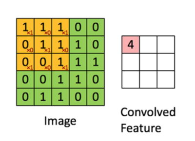
Consider a 5x5 pixel image. For simplicities sake, let’s assume that the pixel values can only take on values 0 or 1. In reality they could take on many values based on the colour scheme, but the operation will be the same. The yellow piece overlaying one part of the image is called a “filter”, and is used to derive the value in the convolved feature. For example: 1*1 + 1*0 + 1*1 + 0*0 + 1*1 + 1*0 + 0*1 + 0*0 + 1*1 = 4. In this example, we set our “stride” parameter to 1. That is, we move the filter matrix to the right by 1 to get the (2,1) element for our convolved feature matrix. Likewise, we move our filter down one to get the (1,2) element of the convolved matrix. A similar operation can be applied to vectors with an nx1 filter.
Step 2: Non-linearity
Next, we apply a non-linear function to the elements of the Convolved Feature in order to account for non-linearity. For example, we might take the function max(element,0) and apply it to the matrix
Step 3: Pooling
In the final step, we divide our convolved matrix into sub-matrices and apply sum summary function to that sub-matrix. For example, we can take the max, min or sum of elements in the sub-matrix as an element in our final matrix.
At the end of this 3 step process, we would have developed a standard vector of features that would then travel through “fully connected layers”. Note that the pooling step is not entirely necessary, but it does help in developing equivariant representations of our image accounting for small distortions in images. The structure with these layers would either be that of a FFNN layer or another “convolution layer”, where the above mentioned 3 step process is applied again to the inputs as the operation for that layer. Below we describe how one would go about training a CNN with Backpropagation.
Backpropagation and Gradient Calculation for Various CNN Components
Backpropagation is the typical method used to train neural networks. It is an extended, systematic application of chain rule, where the the weights of a network are tuned in a series of iterations through adding a multiple of the gradient of the error function w.r.t the weights, to the weights themselves. This corresponds to finding the best direction of change for a neural network’s weights that will result in a locally optimal decrease in the error metric.
Typically, a calculation of the gradient for weights is broken down into the multiplication of individual components of the path from the weight to the final error function, something like E/w = E/a a/z z/w. Backpropagation yields chained gradient (matrix) multiplications, so it is important to know the gradient calculation for each component, whether it is convolution, pooling, matrix multiplication (found in dense layers).
In a typical CNN, there are many different components, and each component warrants its own backpropagation calculation.
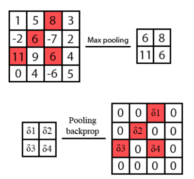
For pooling, lets say 2-d max pooling with stride 2, for example, the output is a multidimensional version of the max of a 2x2 input block. Thus, the backprop step through a max pool layer is simply 1 for whichever input in the 2x2 block is highest, and 0 for the rest. Thus it serves as a selective passthrough for the gradient at certain locations.
(Image from Medium post)
For typical activation like ReLU, which is a multidimensional (elementwise) y=max(0,x), the gradient through the component is simply 1 if x > 0 and 0 otherwise, and is again a selective passthrough of the gradient at certain locations.
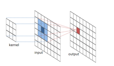
For a convolution layer, assuming 2D convolution, and that input dimension are of dimensions (h,w,c), i.e. height, width, and # of channels, and the output being (h’, w’, k), i.e. output height, width, and # of filters, we know that the the position x,y of the output of filter k is the convolution of a kernel-shaped block of input against the same sized kernel filter (which means to elementwise multiply, and sum across all elements). Thus, the gradient of the layer output w.r.t the layer input is simply the a matrix of copies of the weight and some zeros. Also, the gradient of the layer output w.r.t the weights is simply an aggregation of all the individual input activations that have been multiplied onto the weights in the convolution step.
(Image from Github)
Finally, for fully connected (i.e. dense) layers, the output of a layer is simply a matrix multiplication of the inputs. Thus the gradient of the output w.r.t the input is the weight matrix itself. The gradient of the output w.r.t. Weights are the input activations that have touched the respective elements of the weight matrix during the multiplication step, which is an aggregation of the inputs of the layer.
Through the individual gradients of each component, we can use chain rule to build the gradient of the error w.r.t all weights, and apply these gradients using typical first-order optimization methods like stochastic gradient descent, and variants thereof.


