stat441w18/A New Method of Region Embedding for Text Classification
Presented by
1. Liu, Yanting
2. Huang, Jingyue
3. Wang, Xiaohan
4. Yao, Tangxinxin
5. Li, Kecheng
6. Pan, Lisi
7. Liu, Mingguang
8. Fan, Ming
Introduction
Text classification involves many areas such as topic categorization, sentiment analysis and search query classification. After years of study researchers have developed a number of methods for feature engineering. A simple but effective approach for text classification is the bag-of-words model. That is to represent documents as vectors and train a classifier based on these representations using methods like Support Vector Machines and Naive Bayes. However this kind of model ignores the word order, which is very useful at least in sentiment analysis.
To utilize the order information, people developed N-gram model, which is to predict the Nth word base on the last N-1 words with Markov Chain Model. Yet it still has limitations. For example, as the length N increases the number of parameters becomes large then the estimation suffers from the data sparsity problem.
In this paper, authors proposed to learn the region embedding (following Johnson & Zhang 2015) of n-grams for a specific task. Intuitively the meaning of a word is defined by the meaning of itself and that of words in surrounding context. Therefore, the extended embedding consists of two parts: the embedding of the word itself and a matrix describing its interaction with local context (called local context unit). Then the region embedding of an N-gram is constructed using extended embedding of all words in this N-gram. For the text classification task, documents can then be represented as a bag of region embeddings and we can train a classifier on the basis of these region embeddings.
Related work
FastText FastText uses the word embeddings to represent a document and a fully connected linear layer as the classifier. To make use of order information of small regions it uses hand-crafted n-grams as features in addition to single words.
CNN Convolutional Neural Network is a feed-forward network with convolutional layers. The essence of CNN is to learn word embeddings for small size regions and each kernel of convolutional layer tries to capture a specific semantic or structural feature.
Method
This paper focuses on representing small text regions which can preserve local internal structural information for specific text classification. It defines [math]\displaystyle{ region\left ( i,c\right ) }[/math] as the [math]\displaystyle{ 2\times c+1 }[/math] length region with middle word [math]\displaystyle{ \omega_i }[/math] which is the i-th word of the document. And then it uses word embeddings and the local context units to produce region embedding. In the following, we first introduce local context unit, then two architectures to generate the region embedding, and how to classify text.
Local context unit
The vocabulary is represented by a matrix [math]\displaystyle{ \mathbf{E}\in \mathbb{R}^{h \times v} }[/math] with a look up layer, denoted by the embedding [math]\displaystyle{ e_\omega }[/math]. The i-th column represents the embedding of [math]\displaystyle{ \omega_i }[/math], denoted by [math]\displaystyle{ \mathbf{e}_{\omega_i} }[/math].
For each word [math]\displaystyle{ \omega_i }[/math], we define the local context unit [math]\displaystyle{ \mathbf{K}_{\omega_i}\in \mathbb{R}^{h\times\left (2c+1\right )} }[/math]. Let [math]\displaystyle{ \mathbf{K}_{\omega_i,t} }[/math] be the (c+t)-th column in [math]\displaystyle{ \mathbf{K}_{\omega_i} \left (t \in \left [ -c,c \right ] \right ) }[/math], representing a distinctive linear projection function on [math]\displaystyle{ \mathbf{e}_{c+t} }[/math] in the local context [math]\displaystyle{ r\left (i,c\right ) }[/math]. Thus, we can utilize local ordered word information in terms of each word.
Define [math]\displaystyle{ \mathbf{p}_{\omega_i+t}^i }[/math] as the projected word embedding of [math]\displaystyle{ \omega_i+t }[/math] in i-th word’s view, computed by: [math]\displaystyle{ \mathbf{p}_{\omega_i+t}^i = \mathbf{K}_{\omega_i,t} \odot \mathbf{\omega_{i+t}} }[/math] where [math]\displaystyle{ \odot }[/math] denotes an element-wise multiplication.
Note local context units and embedding are learned as model parameters. Local context units can be learned to capture the semantic and syntactic influence of each word to its context.
Word-context region embedding
We proposed two architectures to perform the region embedding from different perspectives. The first one is word-context region embedding, and the second one is context-word region embedding. In this paper, we consider middle words of the regions, hence we can compose the semantics of a give region only by the middle words influences on the context words, or the context words'influences on the middle word. The most important thing from these two different perspectives in this model is the interaction between words.
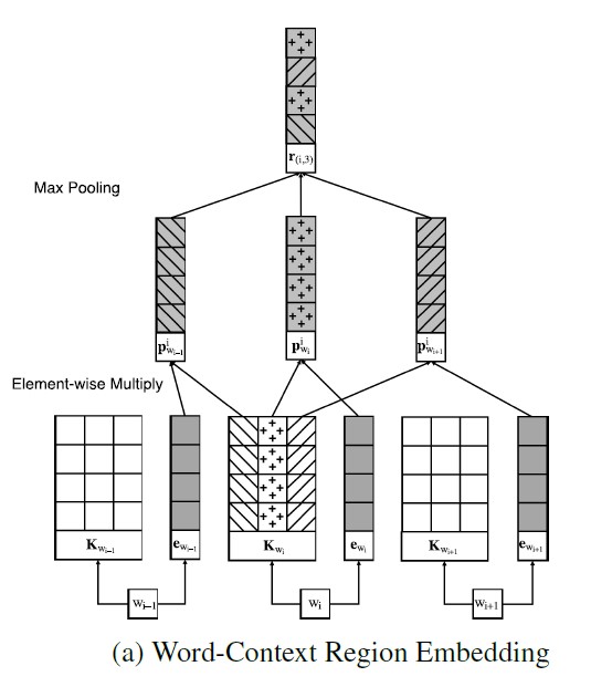
In the first proposed architecture, we focus on addressing the middle word's influences on the context words. For example, in the sentence The food is not very good in this hotel, the occurrence of word not might bring a semantic reversal to the local region.
The figure below is the architecture in a word-context view.
From the bottom to the top, the architecture is,
Step1: Find the middle word [math]\displaystyle{ \omega_{i} }[/math] and choose t from -c to c.
Step2: We use the local context unit of the middle word and the original word embeddings in a region and do element-wise multiply to perform the projected embeddings in a word-to-context view,
[math]\displaystyle{ \mathbf{p}_{w_{i+t}}^i = \mathbf{K}_{\omega_i,t}\cdot\mathbf{e}_{w_{i+t}} }[/math]
where the projected embeddings can reflect the middle word's influences on the context words.
Step3: Once the projected embeddings are obtained, a max pooling operation is applied to extract the most predictive features in the region. The output of the max pooling operation can be regarded as a task related region embedding in a word-to-context view.
[math]\displaystyle{ \mathbf{r}_{\left(i,c\right)}=max\left(\left[\mathbf{p}_{w_{i-c}}^i \ \mathbf{p}_{w_{i-c+1}}^i \cdots \ \mathbf{p}_{w_{i+c-1}}^i \ \mathbf{p}_{w_{i+c}}^i\right]\right) }[/math]
context - Word region embedding
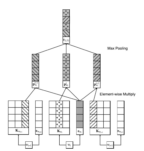
The second architecture goes as a different view, which addresses the local context words’ influences on the middle word in the region, and we call this Context-Word region embedding.
The difference is the projected embeddings are computed by the original word embedding of the middle word and the context units of all words in the region, then the Context-Word region embedding can be obtained by a max pooling operation through the column dimension of the projected embedding matrix:
[math]\displaystyle{ \mathbf{r}_{\left(i,c\right)}=max\left(\left[\mathbf{p}_{w_i}^{i-c} \ \mathbf{p}_{w_i}^{i-c+1} \cdots \ \mathbf{p}_{w_i}^{i+c-1} \ \mathbf{p}_{w_i}^{i+c}\right]\right) }[/math]
Two models take different ways to produce the projected word embeddings, the Word-Context model uses context units of middle words and word embeddings of context words, while the Context-Word model uses context units of context words and word embeddings of the middle word.
Region Embedding For Text Classification
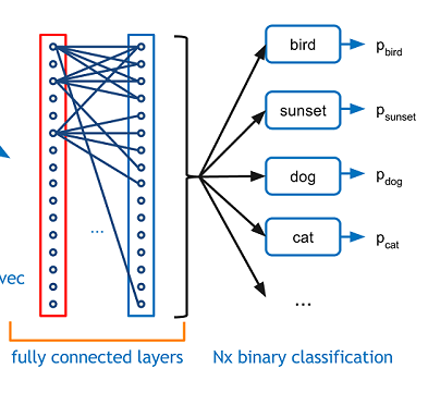
For text classification, documents are usually variable-sized, which need to be represented as fixed size vectors. In order to show the effectiveness of our proposed region embedding models, we just sum up the embeddings of all regions to represent a document, and feed it directly to an Full-Connected layer for text classification task. This layer takes an input volume and outputs an N dimensional vector where N is the number of classes that the program has to choose from. Basically, a FC layer looks at what high level features most strongly correlate to a particular class and has particular weights so that when you compute the products between the weights and the previous layer, you get the correct probabilities for the different classes.
Formally, the model can be represented as following: [math]\displaystyle{ \mathbf{f} (\mathbf{x};\mathbf{E}, \mathbf{U},\mathbf{W},\mathbf{b})= \mathbf{g} (\mathbf{W} \sigma ( \sum_{i=0}^{n} ( r_{(i,c)} ) ) +b) }[/math]
Where [math]\displaystyle{ x }[/math] denotes the input text sequence, [math]\displaystyle{ W }[/math] and [math]\displaystyle{ b }[/math] denote the weight matrix and bias of the fully connected layer respectively. [math]\displaystyle{ n }[/math] denotes the number of regions in a document, [math]\displaystyle{ r }[/math] is the region embedding which can be computed by the equation(2). [math]\displaystyle{ g }[/math] and [math]\displaystyle{ \sigma }[/math] denote the softmax function of the output layer and the softsign function. For soft-sign function: [math]\displaystyle{ \mathbf{y} = \frac{\mathbf{x}} {1+\lVert \mathbf{x} \rVert} }[/math]
For soft-max function: [math]\displaystyle{ \g :\mathbb{R}^{k} \rightarrow \mathbb{ {\left [0,1\right ]}^{k} } }[/math]
Suppose [math]\displaystyle{ h }[/math] is the embedding size and [math]\displaystyle{ k }[/math] is the number of text classification. [math]\displaystyle{ r_{\left (i,c\right )} }[/math] is a [math]\displaystyle{ h \times 1 }[/math] matrix. Also a summation of embedding of all regions in one document [math]\displaystyle{ \sum_{i=0}^{n} ( r_{\left (i,c\right )} ) }[/math] has the same dimension and After the soft-sign function, [math]\displaystyle{ \sigma ( \sum_{i=0}^{n} ( r_{\left (i,c\right )} ) ) }[/math] is also a [math]\displaystyle{ h \times 1 }[/math] matrix. The weight matrix [math]\displaystyle{ W }[/math] is [math]\displaystyle{ k \times h }[/math]. The bias of FC layers [math]\displaystyle{ b }[/math] measures the difference between final output and the real results, so it is [math]\displaystyle{ k \times 1 }[/math] matrix. So, [math]\displaystyle{ \mathbf{W} \sigma ( \sum_{i=0}^{n} ( r_{(i,c)} ) ) +b }[/math] becomes [math]\displaystyle{ k \times 1 }[/math]. Finally, After soft-max function transformation, the range is transformed into [0,1]. The object function finally becomes [math]\displaystyle{ k \times 1 }[/math]. Which measures the document’s probabilities that belong to each class. At the beginning, we can set the initial value which is very close to 0 to Weight Matrix, and we can get the initial value of bias of FC layer at the first output. Just as the same mechanism in the Backpropagation Neutral Network, We can update the weight matrix and bias matrix in the training period until we get the optimal.
Experiments
Introduction
The experiment in the paper uses the publicly available datasets from Zhang et al. (2015) to evaluate the model. The results are compared with those using several other methods including n-grams, ngrams TFIDF, char-CNN, char-CRNN, bigram-FastText, VDCVV and D-LSTM.
Process
Firstly, all the texts are tokenized. As for the parameters in the model, optimal hyperparameters are obtained by tuning with 10% of the training set on Yep Review Full dataset. The initial values are assigned to the identical hyperparameters, where the dimension of word embedding is 128 and the region size is 7. In the meantime, the initial learning rate is set to 0.0001 and the batch size is 16. The region size and embedding size are chosen based on following two experiments.
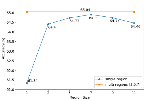
Figure 1 shows the relationship between different region sizes and accuracy. For single region, when region size equals to 7, the accuracy is the highest. However, adding the multi region of the combination of 3, 5 and 7, it yields to the highest accuracy. It is easy to be understood since the influence ranges between words can differ a lot. For example, the word “very” only emphasizes the next word while the word like “however” might have influence on a lot of following words.
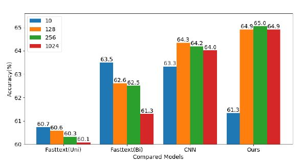
Figure 2 shows the accuracy based on different embedding dimensions and different models. The change of accuracy shows the model proposed in this paper is more robust to overfitting compared with FastText and CNN.
Results
The table below shows all the results for the ten different methods on the eight datasets.
Table 1: Test Set Accuracy [%] Compared to other Methods on several Datasets
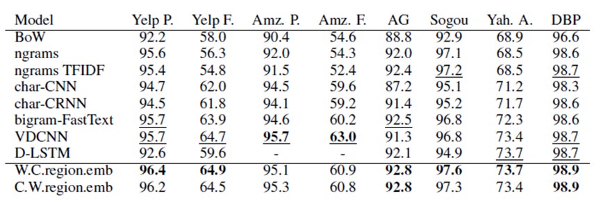
In this table, underscores is used to represent the best published results, and the best records is bolded. The model proposed in this paper wins all the previous models on all datasets except for using VDCNN on Amz.P. and Amz.F.
Analyzing the performance of this model, consideration of context unit plays an important role. Some comparative experiments are explored to show the effectiveness of the proposed word specific context unit.
Table 2: Comparative decomposition results on Yelp Review Full dataset. For Fast-Text(Unigram), embedding dimension is 10. For FastText(Win-pool), W.C.region.emb(Scalar) and W.C.region.emb(our model), region size is 7 and embedding dimension is 128

The FastText(Unigram) model is the baseline model. The FastText(Win-pool) model is established by removing the entire context units from the model proposed by this paper, which is a variant version of unigram FastText. Then after applying a simplified scalar version of context units to FastText(Win-pool), the model W.C.region.emb(Scalar) can be acquired. Finally W.C.region.emb(our model) is the variant version of W.C.region.emb(Scalar), where each column of scalar context unit is expanded to a dense vector. From the table above, it can be seen that the consideration of context unit can improve the model significantly.
Conclusion
The paper proposed two new methods for text classification called Word-Context Region Embedding and Context-Word Region Embedding. The experiments show the accuracy of text classification has improved a lot compared with the previous methods. However, the current result might be improved by introducing more complex upper layers. The power of the local context unit also needs to be tested under unsupervised and semi-supervised learning.
