Understanding Image Motion with Group Representations

Introduction

Motion perception is a key component of computer vision. It is critical to problems such as optical flow and visual odometry, where a sequence of images are used to calculate either the pixel level (local) motion or the motion of the entire scene (global). The smooth image transformation caused by camera motion is a subspace of all position image transformations. Here, we are interested in realistic transformation caused by motion, therefore unrealistic motion caused by say, face swapping, are not considered.

Supervised learning of 3D motion is challenging since explicit motion labels are no trivial to obtain. The proposed learning method does not need label data. Instead, the method constrains learning by using the properties of motion space. The paper presents a general model of visual motion, and how the motion space properties of associativity and invertibility can be used to constrain the learning of a deep neural network. The results show evidence that the learned model captions motion in both 2D and 3D settings.

Related Work

The most common global representations of motion are from structure from motion (SfM) and simultaneous localization and mapping (SLAM), which represent poses in special Euclidean group [math]\displaystyle{ SE(3) }[/math] to represent a sequence of motions. However, these cannot be used to represent non-rigid or independent motions. Another approach to representing motion is spatiotemporal features (STFs), which are flexible enough to represent non-rigid motions.

There are also works using CNN’s to learn optical flow using brightness constancy assumptions, and/or photometric local constraints. Works on stereo depth estimation using learning has also shown results. Regarding image sequences, there are works on shuffling the order of images to learn representations of its contents, as well as learning representations equivariant to the egomotion of the camera.

Approach

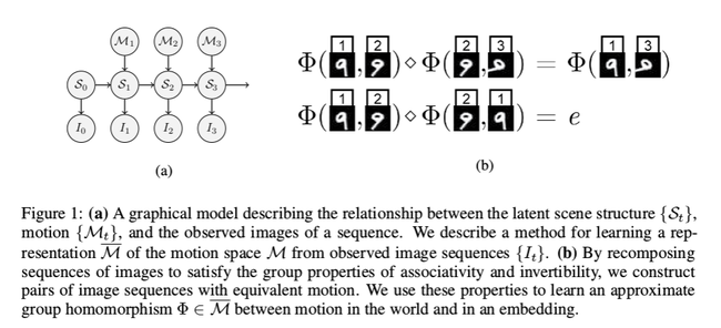
The proposed method is based on the observation that 3D motions, equipped with composition, form a group. By learning the underlying mapping that captures the motion transformations, we are approximating latent motion of the scene. The method is designed to capture group associativity and invertibility.

Consider a latent structure space [math]\displaystyle{ S }[/math], element of the structure space generates images via projection [math]\displaystyle{ \pi:S\rightarrow I }[/math], latent motion space [math]\displaystyle{ M }[/math] which is some closed subgroup of the set of homeomorphism on [math]\displaystyle{ S }[/math]. For [math]\displaystyle{ s \in S }[/math], a continuous motion sequence [math]\displaystyle{ \{m_t \in M | t \geq 0\} }[/math] generates continous image sequence [math]\displaystyle{ \{i_t \in I | t \geq 0\} }[/math] where [math]\displaystyle{ i_t=\pi(m_t(s)) }[/math]. Writing this as a hidden Markov model gives [math]\displaystyle{ i_t=\pi(m_{\Delta t}(s_{t-1}))) }[/math] where the current state is based on the change from the previous. Since [math]\displaystyle{ M }[/math] is a closed group on [math]\displaystyle{ S }[/math], it is associative, has inverse, and contains idenity. [math]\displaystyle{ SE(3) }[/math] is an exmaple of this. To be more specific, the latent structure of a scene from rigid image motion could be modelled by a point cloud with a motion space [math]\displaystyle{ M=SE(3) }[/math], where rigid image motion can be produced by a camera translating and rotating through a rigid scene in 3D. When a scene has N rigid bodies, the motion space can be represented as [math]\displaystyle{ M=[SE(3)]^N }[/math].

Learning Motion by Group Properties

The goal is to learn a function [math]\displaystyle{ \Phi : I \times I \rightarrow \overline{M} }[/math], [math]\displaystyle{ \overline{M} }[/math] indicating representation of [math]\displaystyle{ M }[/math], as well as the composition operator [math]\displaystyle{ \diamond : \overline{M} \rightarrow \overline{M} }[/math] that represents composition in [math]\displaystyle{ M }[/math]. For all sequences, it is assumed that for all times [math]\displaystyle{ t_0 \lt t_1 \lt t_2 ... }[/math], the sequence representation should have the following properties:

1. Associativity: [math]\displaystyle{ \Phi(I_{t_0}, I_{t_1}) \diamond \Phi(I_{t_2}, I_{t_3}) = (\Phi(I_{t_0}, I_{t_1}) \diamond \Phi(I_{t_1}, I_{t_2})) \diamond \Phi(I_{t_2}, I_{t_3}) = \Phi(I_{t_0}, I_{t_1}) \diamond (\Phi(I_{t_1}, I_{t_2}) \diamond \Phi(I_{t_2}, I_{t_3})) = \Phi(I_{t_0}, I_{t_1}) \diamond \Phi(I_{t_1}, I_{t_3}) }[/math], which means that the motion of differently composed subsequences of a sequence are equivalent
2. Has Identity: [math]\displaystyle{ \Phi(I_{t_0}, I_{t_1}) \diamond e = \Phi(I_{t_0}, I_{t_1}) = e \diamond \Phi(I_{t_0}, I_{t_1}) }[/math] and [math]\displaystyle{ e=\Phi(I_{t}, I_{t}) \forall t }[/math], where [math]\displaystyle{ e }[/math] is the null image motion and the unique identity in the latent space
3. Invertibility: [math]\displaystyle{ \Phi(I_{t_0}, I_{t_1}) \diamond \Phi(I_{t_1}, I_{t_0}) = e }[/math], so the inverse of the motion of an image sequence is the motion of that image sequence reversed

An embedding loss is used to approximately enforce associativity and invertibility among subsequences sampled from image sequence. Associativity is encouraged by pushing sequences with the same final motion but different transitions to the same representation. Invertibility is encouraged by pushing sequences corresponding to the same motion with but in opposite directions away from each other, as well as pushing all loops to the same representation. Uniqueness of the identity is encouraged by pushing loops away from non-identity representations. Loops from different sequences are also pushed to the same representation (the identity).

These constraints are true to any type of transformation resulting from image motion. This puts little restriction on the learning problems and allows all features relevant to the motion structure to be captured. On the other hand, optical flow assumes unchanging brightness between frames of the same projected scene, and motion estimates would degrade when that assumption does not hold.

Also with this method, it is possible multiple representations [math]\displaystyle{ \overline{M} }[/math] can be learned from a single [math]\displaystyle{ M }[/math], thus the learned representation is not necessary unique. In addition, the scenes are not expected to have rapid changing content, scene cuts, or long-term occlusions.

Sequence Learning with Neural Networks

The functions [math]\displaystyle{ \Phi }[/math] and [math]\displaystyle{ \diamond }[/math] are approximated by CNN and RNN, respectively. LSTM is used for RNN. The input to the network is a sequence of images [math]\displaystyle{ I_t = \{I_1,...,I_t\} }[/math]. The CNN processes pairs of images are intermediate representations, and the LSTM operates over the sequence of CNN outputs to produce an embedding sequence [math]\displaystyle{ R_t = \{R_{1,2},...,R_{t-1,t}\} }[/math]. Only the embedding at the final time step is used for loss. The network is trained to minimize a hinge loss with respect to embeddings to pairs of sequences as defined below:

[math]\displaystyle{ L(R^1,R^2) = \begin{cases} d(R^1,R^2), & \text{if positive pair} \\ max(0, m - d(R^1,R^2)), & \text{if negative pair} \end{cases} }[/math] [math]\displaystyle{ d_{cosine}(R^1,R^2)=1-\frac{\langle R^1,R^2 \rangle}{\lVert R^1 \rVert \lVert R^2 \rVert} }[/math]

where [math]\displaystyle{ d(R^1,R^2) }[/math] measure the distance between the embeddings of two sequences used for training selected to be cosine distance, [math]\displaystyle{ m }[/math] is a fixed margin selected to be 0.5. Positive pairs are training examples where two sequences have the same final motion, negative pairs are training examples where two sequences have the exact opposite final motion. Using L2 distances yields similar results as cosine distances.

Each training sequence is recomposed into 6 subsequences: two forward, two backward, and two identity. To prevent the network from only looking at static differences, subsequence pairs are sampled such that they have the same start and end frames but different motions in between. Sequences of varying lengths are also used to generalize motion on different temporal scales. Training the network with only one input images per time step was also tried, but consistently yielded work results than image pairs.

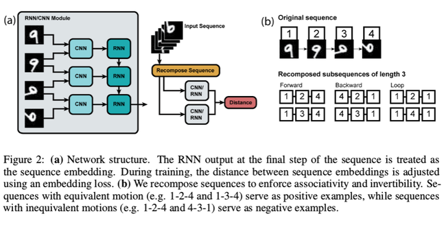
Overall, training with image pairs resulted in lower error than training with just single images. This is demonstrated in the below table.

Experimentation

Trained network using rotated and translated MNIST dataset as well as KITTI dataset.

• Used Torch
• Used Adam for optimization, decay schedule of 30 epochs, learning rate chosen by random serach
• 50-60 batch size for MNIST, 25-30 batch size for KITTI
• Dilated convolution with Relu and batch normalization
• Two LSTM cell per layer 256 hidden units each
• Sequence length of 3-5 images

Rigid Motion in 2D

• MNIST data rotated [math]\displaystyle{ [0, 360) }[/math] degrees and translated [math]\displaystyle{ [-10, 10] }[/math] pixels, i.e. [math]\displaystyle{ SE(2) }[/math] transformations
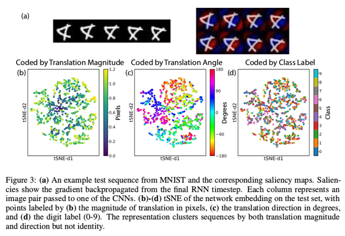
• Visualized the representation using t-SNE
  • Clear clustering by translation and rotation but not object classes
  • Suggests the representation captures the motion properties in the dataset, but is independent of image contents
• Visualized the image-conditioned saliency maps
  • In Figure 3, the red represents the positive gradients of the activation function with respect to the input image, and the negative gradients are represented in blue.
  • If we consider a saliency map as a first-order Taylor expansion, then the map could show the relationship between pixel and the representation.
  • Take derivative of the network output respect to the map
  • The area that has the highest gradient means that part contributes the most to the output
  • The resulting salient map strongly resembles spatiotemporal energy filters of classical motion processing
  • Suggests the network is learn the right motion structure

Real World Motion in 3D

• Uses KITTI dataset collected on a car driving through roads in Germany
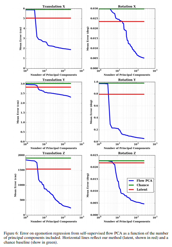
• On a separate dataset with ground truth camera pose, linearly regress the representation to the ground truth
  • The result is compared against self supervised flow algorithm Yu et al.(2016) after the output from the flow algorithm is downsampled, then feed through PCA, then regressed against the camera motion
  • The data shows it performs not as well as the supervised algorithm, but consistently better than chance (guessing the mean value)
  • Shows the method is able to capture dominant motion structure
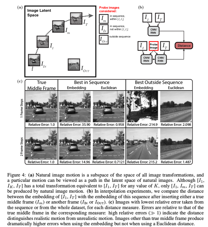
• Test performance on interpolation task
  • Check [math]\displaystyle{ R([I_1,I_T]) }[/math] against [math]\displaystyle{ R([I_1, I_m, I_T]) }[/math], [math]\displaystyle{ R([I_1, I_{IN}, I_T]) }[/math], and [math]\displaystyle{ R([I_1, I_{OUT}, I_T]) }[/math]
  • Test how sensitive the network is to deviations from unnatural motion
  • High errors [math]\displaystyle{ \gg 1 }[/math] means the network can distinguish between realistic and unrealistic motion
  • In order to do this, the distance between the embeddings of the frame sequences of the first and last frame [math]\displaystyle{ R([I_1,I_T]) }[/math] and of the first, middle, and last frame [math]\displaystyle{ R([I_1, I_m, I_T]) }[/math] is computed. This distance is compared with the distance when the middle frame of the second embedding is changed to a frame that is visually similar (inside sequence): [math]\displaystyle{ R([I_1, I_{IN}, I_T]) }[/math] and one that is visually dissimilar (outside sequence): [math]\displaystyle{ R([I_1, I_{OUT}, I_T]) }[/math]. The results are shown in Table 3. The embedding distance method is compared to the Euclidean distance which is defined as the mean pixel distance between the test frame and [math]\displaystyle{ {I_1,I_T} }[/math], whichever is smaller. It can be seen from the results that the embedding distance of the true frame is significantly lower than other frames. This means that the embedding distance used in the network is more sensitive to any atypical motions of the scenes.
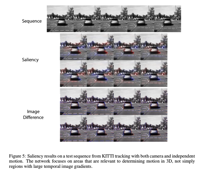
• Visualized saliency maps
  • Highlights objects moving in the background, and motion of the car in the foreground
  • Suggests the method can be used for tracking as well

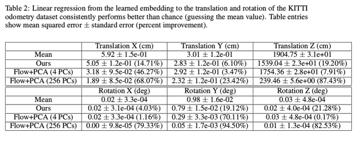
• Figure 7 displays graphs comparing the mean squared error of the method presented in this paper to the baseline chance method and the supervised Flow PCA method.

Conclusion

The author presented a new model of motion and a method for learning motion representations. It is shown that by enforcing group properties we can learn motion representations that are able to generalize between scenes with disparate content. The results can be useful for navigation, prediction, and other behavioral tasks relying on motion. Due to the fact that this method does not require labelled data, it can be applied to a large variety of tasks.

Criticism

Although this method does not require any labelled data, it is still learning by supervision through defined constraints. The idea of training using unlabelled data is interesting and it does have meaningful practical application. Unfortunately, the author did not provide convincing experimental results. Results from motion estimation problems are typically compared against ground truth data for their accuracy. The author performed experiments on transformed MNIST data and KITTI data. The MNIST data is transformed by the author, thus the ground truth is readily available. However the author only claimed the validity of the results through indirect means of using t-SNE and saliency map visualization. For the KITTI dataset, the author regressed the representations against ground truth for some mapping from the network output to some physical motion representation. Again, the results were compared only indirectly against ground truth. Such experimentation made the method hardly convincing and applicable to real world applications. In addition, the network does not output motion representations with physical meanings, make the proposed method useless for any real world applications.

Another criticism is that the group-properties constraint the authors impose is too weak. Any set consisting of functions, their inverses, and the identity forms a group. While physical motions are one example of such a group, there are many valid groups that do not represent any coherent physical motions.

References

Jaegle, A. (2018). Understanding image motion with group representations . ICLR. Retrieved from https://openreview.net/pdf?id=SJLlmG-AZ.

Karen Simonyan, Andrea Vedaldi, and Andrew Zisserman. Deep inside convolutional networks: Visualising image classification models and saliency maps. In International Conference on Learning Representations (ICLR) Workshop, 2013.

Jason J Yu, Adam W Harley, and Konstantinos G Derpanis. Back to basics: Unsupervised learning of optical flow via brightness constancy and motion smoothness. European Conference on Computer Vision (ECCV) Workshops, 2016.