stat946w18/Unsupervised Machine Translation Using Monolingual Corpora Only
Introduction
Neural machine translation systems are usually trained on large corpora consisting of pairs of pre-translated sentences. The paper Unsupervised Machine Translation Using Monolingual Corpora Only by Guillaume Lample, Ludovic Denoyer, and Marc'Aurelio Ranzato proposes an unsupervised neural machine translation system, which can be trained without such parallel data.
Motivation
The authors offer two motivations for their work:
- To translate between languages for which large parallel corpora does not exist
- To provide a strong lower bound that any semi-supervised machine translation system is supposed to yield
Overview of unsupervised translation system
The unsupervised translation scheme has the following outline:
- The word-vector embeddings of the source and target languages are aligned in an unsupervised manner.
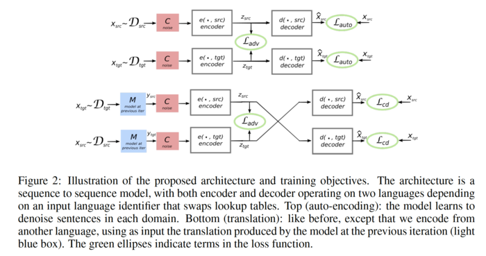
- Sentences from the source and target language are mapped to a common latent vector space by an encoder, and then mapped to probability distributions over sentences in the target or source language by a decoder.
- A de-noising auto-encoder loss encourages the latent-space representations to be insensitive to noise.
- An adversarial loss encourages the latent-space representations of source and target sentences to be indistinguishable from each other. It is intended that the latent-space representation of a sentence should reflect its meaning, and not the particular language in which it is expressed.
- A reconstruction loss encourages the model to improve on the translation model of the previous epoch.

Notation
Let [math]\displaystyle{ S }[/math] denote the set of words in the source language, and let [math]\displaystyle{ T }[/math] denote the set of words in the target language. Let [math]\displaystyle{ H \subset \mathbb{R}^{n_H} }[/math] denote the latent vector space. Moreover, let [math]\displaystyle{ S' }[/math] and [math]\displaystyle{ T' }[/math] denote the sets of finite sequences of words in the source and target language, and let [math]\displaystyle{ H' }[/math] denote the set of finite sequences of vectors in the latent space. For any set X, elide measure-theoretic details and let [math]\displaystyle{ \mathcal{P}(X) }[/math] denote the set of probability distributions over X.
Word vector alignment
Conneau et al. (2017) describe an unsupervised method for aligning word vectors across languages. By "alignment", I mean that their method maps words with related meanings to nearby vectors, regardless of the language of the words. Moreover, if two words are one another's literal translations, their word vectors tend to be mutual nearest neighbors.
The underlying idea of the alignment scheme can be summarized as follows: methods like word2vec or GLoVe generate vectors for which there is a correspondence between semantics and geometry. If [math]\displaystyle{ f }[/math] maps English words to their corresponding vectors, we have the approximate equation \begin{align} f(\text{king}) -f(\text{man}) +f(\text{woman})\approx f(\text{queen}). \end{align} Furthermore, if [math]\displaystyle{ g }[/math] maps French words to their corresponding vectors, then \begin{align} g(\text{roi}) -g(\text{homme}) +g(\text{femme})\approx g(\text{reine}). \end{align}
Thus if [math]\displaystyle{ W }[/math] maps the word vectors of English words to the word vectors of their French translations, we should expect [math]\displaystyle{ W }[/math] to be linear. As was observed by Mikolov et al. (2013), the problem of word-vector alignment then becomes a problem of learning the linear transformation that best aligns two point clouds, one from the source language and one from the target language. For more on the history of the word-vector alignment problem, see my CS698 project (link).
Conneau et al. (2017)'s word vector alignment scheme is unique in that it requires no parallel data, and uses only the shapes of the two word-vector point clouds to be aligned. I will not go into detail, but the heart of the method is a special GAN, in which only the discriminator is a neural network, and the generator is the map corresponding to an orthogonal matrix.
This unsupervised alignment method is crucial to the translation scheme of the current paper. From now on we denote by [math]\displaystyle{ A: S' \cup T' \to \mathcal{Z}' }[/math] the function that maps a source- or target- language word sequence to the corresponding aligned word vector sequence.
Encoder
The encoder [math]\displaystyle{ E }[/math] reads a sequence of word vectors [math]\displaystyle{ (z_1,\ldots, z_m) \in \mathcal{Z}' }[/math] and outputs a sequence of hidden states [math]\displaystyle{ (h_1,\ldots, h_m) \in H' }[/math] in the latent space. Crucially, because the word vectors of the two languages have been aligned, the same encoder can be applied to both. That is, to map a source sentence [math]\displaystyle{ x=(x_1,\ldots, x_M)\in S' }[/math] to the latent space, we compute [math]\displaystyle{ E(A(x)) }[/math], and to map a target sentence [math]\displaystyle{ y=(y_1,\ldots, y_K)\in T' }[/math] to the latent space, we compute [math]\displaystyle{ E(A(y)) }[/math].
The encoder consists of two LSTMs, one of which reads the word-vector sequence in the forward direction, and one of which reads it in the backward direction. The hidden state sequence is generated by concatenating the hidden states produced by the forward and backward LSTMs at each word vector.
Decoder
The decoder is a mono-directional LSTM that accepts a sequence of hidden states [math]\displaystyle{ h=(h_1,\ldots, h_m) \in H' }[/math] from the latent space and a language [math]\displaystyle{ L \in \{S,T \} }[/math] and outputs a probability distribution over sentences in that language. We have
\begin{align} D: H' \times \{S,T \} \to \mathcal{P}(S') \cup \mathcal{P}(T'). \end{align}
The decoder makes use of the attention mechanism of Bahdanau et al. (2014). To compute the probability of a given sentence [math]\displaystyle{ y=(y_1,\ldots,y_K) }[/math] , the LSTM processes the sentence one word at a time, accepting at step [math]\displaystyle{ k }[/math] the aligned word vector of the previous word in the sentence [math]\displaystyle{ A(y_{k-1}) }[/math] and a context vector [math]\displaystyle{ c_k\in H }[/math] computed from the hidden sequence [math]\displaystyle{ h\in H' }[/math], and outputting a probability distribution over possible next words. The LSTM is initiated with a special, language-specific start-of-sequence token. Otherwise, the decoder is does not depend on the language of the sentence it is producing. The context vector is computed as described by Bahdanau et al. (2014), where we let [math]\displaystyle{ l_{k} }[/math] denote the hidden state of the LSTM at step [math]\displaystyle{ k }[/math], and where [math]\displaystyle{ U,W }[/math] are learnable weight matrices, and [math]\displaystyle{ v }[/math] is a learnable weight vector: \begin{align} c_k&= \sum_{m=1}^M \alpha_{k,m} h_m\\ \alpha_{k,m}&= \frac{\exp(e_{k,m})}{\sum_{m'=1}^M\exp(e_{k,m'}) },\\ e_{k,m} &= v^T \tanh (Wl_{k-1} + U h_m ). \end{align}
By learning [math]\displaystyle{ U,W }[/math] and [math]\displaystyle{ v }[/math], the decoder can learn to decide which vectors in the sequence [math]\displaystyle{ h }[/math] are relevant to computing which words in the output sentence.
At step [math]\displaystyle{ k }[/math], after receiving the context vector [math]\displaystyle{ c_k\in H }[/math] and the aligned word vector of the previous word in the sequence,[math]\displaystyle{ A(y_{k-1}) }[/math], the LSTM outputs a probability distribution over words, which should be interpreted as the distribution of the next word according to the decoder. The probability the decoder assigns to a sentence is then the product of the probabilities computed for each word in this manner.
Overview of objective
The objective function is the sum of:
- The de-noising auto-encoder loss,
- The translation loss,
- The adversarial loss.
I shall describe these in the following sections.
De-noising Auto-encoder Loss
A de-noising auto-encoder is a function optimized to map a corrupted sample from some dataset to the original un-corrupted sample. De-noising auto-encoders were introduced by Vincent et al. (2008), who provided numerous justifications, one of which is particularly illuminating. If we think of the dataset of interest as a thin manifold in a high-dimensional space, the corruption process is likely perturbed a datapoint off the manifold. To learn to restore the corrupted datapoint, the de-noising auto-encoder must learn the shape of the manifold.
Hill et al. (2016), used a de-noising auto-encoder to learn vectors representing sentences. They corrupted input sentences by randomly dropping and swapping words, and then trained a neural network to map the corrupted sentence to a vector, and then map the vector to the un-corrupted sentence. Interestingly, they found that sentence vectors learned this way were particularly effective when applied to tasks that involved generating paraphrases. This makes some sense: for a vector to be useful in restoring a corrupted sentence, it must capture something of the sentence's underlying meaning.
The present paper uses the principal of de-noising auto-encoders to compute one of the terms in its loss function. In each iteration, a sentence is sampled from the source or target language, and a corruption process [math]\displaystyle{ C }[/math] is applied to it. [math]\displaystyle{ C }[/math] works by deleting each word in the sentence with probability [math]\displaystyle{ p_C }[/math] and applying to the sentence a permutation randomly selected from those that do not move words more than [math]\displaystyle{ k_C }[/math] spots from their original positions. The authors select [math]\displaystyle{ p_C=0.1 }[/math] and [math]\displaystyle{ k_C=3 }[/math]. The corrupted sentence is then mapped to the latent space using [math]\displaystyle{ E\circ A }[/math]. The loss is then the negative log probability of the original un-corrupted sentence according to the decoder [math]\displaystyle{ D }[/math] applied to the latent-space sequence.
The explanation of Vincent et al. (2008) can help us understand this loss-function term: the de-noising auto-encoder loss forces the translation system to learn the shapes of the manifolds of the source and target languages.
Translation Loss
To compute the translation loss, we sample a sentence from one of the languages, translate it with the encoder and decoder of the previous epoch, and then corrupt its output with [math]\displaystyle{ C }[/math]. We then use the current encoder [math]\displaystyle{ E }[/math] to map the corrupted translation to a sequence [math]\displaystyle{ h \in H' }[/math] and the decoder [math]\displaystyle{ D }[/math] to map [math]\displaystyle{ h }[/math] to a probability distribution over sentences. The translation loss is the negative log probability the decoder assigns to the original uncorrupted sentence.
It is interesting and useful to consider why this translation loss, which depends on the translation model of the previous iteration, should promote an improved translation model in the current iteration. One loose way to understand this is to think of the translator as a de-noising translator. We are given a sentence perturbed from the manifold of possible sentences from a given language both by the corruption process and by the poor quality of the translation. The model must learn to both project and translate. The technique employed here resembles that used by Sennrich et al. (2014), who trained a neural machine translation system using both parallel and monolingual data. To make use of the monolingual target-language data, they used an auxiliary model to translate it to the source language, then trained their model to reconstruct the original target-language data from the source-language translation. Sennrich et al. argued that training the model to reconstruct true data from synthetic data was more robust than the opposite approach. The authors of the present paper use similar reasoning.
Adversarial Loss
The intuition underlying the latent space is that it should encode the meaning of a sentence in a language-independent way. Accordingly, the authors introduce an adversarial loss, to encourage latent-space vectors mapped from the source and target languages to be indistinguishable. Central to this adversarial loss is the discriminator [math]\displaystyle{ R:H' \to [0,1] }[/math], which makes use of [math]\displaystyle{ r: H\to [0,1] }[/math] a three-layer fully-connected neural network with 1024 hidden units per layer. Given a sequence of latent-space vectors [math]\displaystyle{ h=(h_1,\ldots,h_m)\in H' }[/math] the discriminator assigns probability [math]\displaystyle{ R(h)=\prod_{i=1}^m r(h_i) }[/math] that they originated in the target space. Each iteration, the discriminator is trained to maximize the objective function
\begin{align} I_T(q) \log (R(E(q))) +(1-I_T(q) )\log(1-R(E(q))) \end{align}
where [math]\displaystyle{ q }[/math] is a randomly selected sentence, and [math]\displaystyle{ I_T(q) }[/math] is 1 when [math]\displaystyle{ q\in I_T }[/math] is from the source language and 0 if [math]\displaystyle{ q\in I_S }[/math]
The same term is added to the primary objective function, which the encoder and decoder are trained to minimize. The result is that the encoder and decoder learn to fool the discriminator by mapping sentences from the source and target language to similar sequences of latent-space vectors.
The authors note that they make use of label smoothing, a technique recommended by Goodfellow (2016) for regularizing GANs, in which the objective described above is replaced by
\begin{align} I_T(q)( (1-\alpha)\log (R(E(q))) +\alpha\log(1-R(E(q))) )+(1-I_T(q) ) ( (1-\beta) \log(1-R(E(q))) +\beta\log (R(E(q)) )) \end{align} for some small nonnegative values of [math]\displaystyle{ \alpha, \beta }[/math], the idea being to prevent the discriminator from making extreme predictions. While one-sided label smoothing ([math]\displaystyle{ \beta = 0 }[/math]) is generally recommended, the present model differs from a standard GAN in that it is symmetric, and hence two-sided label smoothing would appear more reasonable.
It is interesting to observe that while the intuition justifying the use of the latent space suggests that the latent space representation of a sentence should be language-independent, this is not actually true: if two sentences are translations of one another, but have different lengths, their latent-space representations will necessarily be different, since a a sentence's latent space representation has the same length as the sentence itself.
Objective Function
Combining the above-described terms, we can write the overall objective function. Let [math]\displaystyle{ Q_S }[/math] denote the monolingual dataset for the source language, and let [math]\displaystyle{ Q_T }[/math] denote the monolingual dataset for the target language. Let [math]\displaystyle{ D_S:= D(\cdot, S) }[/math] and[math]\displaystyle{ D_T= D(\cdot, T) }[/math] (i.e. [math]\displaystyle{ D_S, D_T }[/math]) be the decoder restricted to the source or target language, respectively. Let [math]\displaystyle{ M_S }[/math] and [math]\displaystyle{ M_T }[/math] denote the target-to-source and source-to-target translation models of the previous epoch. Then our objective function is
\begin{align} \mathcal{L}(D,E,R)=\text{T Translation Loss}+\text{T De-noising Loss} +\text{T Adversarial Loss} +\text{S Translation Loss} +\text{S De-noising Loss} +\text{S Adversarial Loss}\\ \end{align} \begin{align} =\sum_{q\in Q_T}\left( -\log D_T \circ E \circ C \circ M _S(q) (q) -\log D_T \circ E \circ C (q) (q)+(1-\alpha)\log (R\circ E(q)) +\alpha\log(1-R\circ E(q)) \right)+\sum_{q\in Q_S}\left( -\log D_S \circ E \circ C \circ M_T (q) (q) -\log D_S \circ E \circ C (q) (q)+(1-\beta) \log(1-R \circ E(q)) +\beta\log (R\circ E(q) \right). \end{align}
They alternate between iterations minimizing [math]\displaystyle{ \mathcal{L} }[/math] with respect to [math]\displaystyle{ E, D }[/math] and iterations maximizing with respect to [math]\displaystyle{ R }[/math]. ADAM is used for minimization, while RMSprop is used for maximization. After each epoch, M is updated so that [math]\displaystyle{ M_S=D_S \circ E }[/math] and [math]\displaystyle{ M_T=D_T \circ E }[/math], after which [math]\displaystyle{ M }[/math] is frozen until the next epoch.
Validation
The authors' aim is for their method to be completely unsupervised, so they do not use parallel corpora even for the selection of hyper-parameters. Instead, they validate by translating sentences to the other language and back, and comparing the resulting sentence with the original according to BLEU, a similarity metric frequently used in translation (Papineni et al. 2002).
Experimental Procedure and Results
The authors test their method on four data sets. The first is from the English-French translation task of the Workshop on Machine Translation 2014 (WMT14). This data set consists of parallel data. The authors generate a monolingual English corpus by randomly sampling 15 million sentence pairs, and choosing only the English sentences. They then generate a French corpus by selecting the French sentences from those pairs that were not previous chosen. Importantly, this means that the monolingual data sets have no parallel sentences. The second data set is generated from the English-German translation task from WMT14 using the same procedure.
The third and fourth data sets are generated from Multi30k data set, which consists of multilingual captions of various images. The images are discarded and the English, French, and German captions are used to generate monolingual data sets in the manner described above. These monolingual corpora are much smaller, consisting of 14500 sentences each.
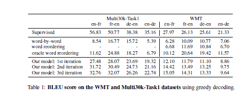
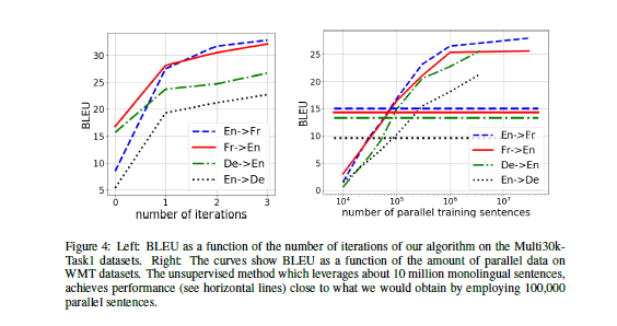
The unsupervised translation scheme performs well, though not as well as a supervised translation scheme. It converges after a small number of epochs. Besides supervised translation, the authors compare their method with three other baselines: "Word-by-Word" uses only the previously-discussed word-alignment scheme; "Word-Reordering" uses a simple LSTM based language model and a greedy algorithm to select a reordering of the words produced by "Word-by-Word". "Oracle Word Reordering" means the optimal reordering of the words produced by "Word-by-Word".
Result Figures
Commentary
This paper's results are impressive: that it is even possible to translate between languages without parallel data suggests that languages are more similar than we might initially suspect, and that the method the authors present has, at least in part, discovered some common deep structure. As the authors point out, using no parallel data at all, their method is able to produce results comparable to those produced by neural machine translation methods trained on hundreds of thousands of a parallel sentences on the WMT dataset. On the other hand, the results they offer come with a few significant caveats.
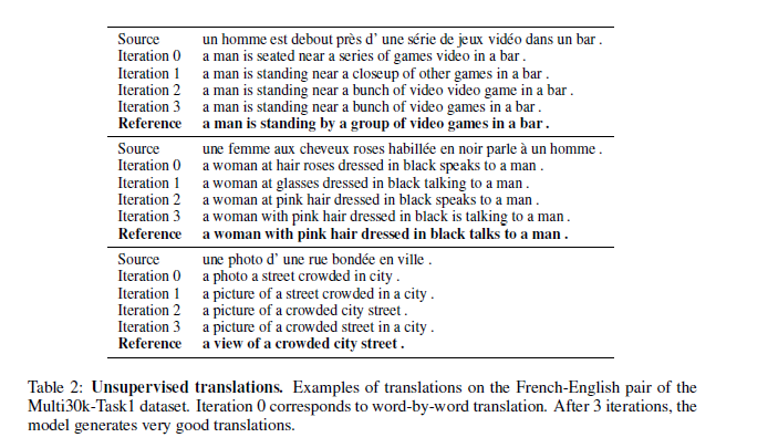
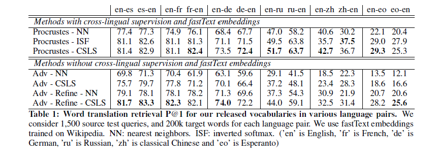
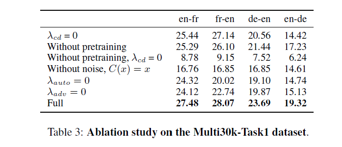
The first caveat is that the workhorse of the method is the unsupervised word-vector alignment scheme presented in Conneau et al. (2017) (that paper shares 3 authors with this one). As the ablation study reveals, without word-vector alignment, this method preforms extremely poorly. Moreover, word-by-word translation using word-vector alignment alone performs well, albeit not as well as this method. This suggests that the method of this paper mainly learns to perform (sometimes significant) corrections to word-by-word translations by reordering and occasional word substitution. Presumably, it does this by learning something of the natural structure of sentences in each of the two languages, so that it can correct the errors made by word-by-word translation.
The second caveat is that the best results are attained translating between English and French, two very closely related languages, and the quality of translation between English and German, a slightly-less related pair, is significantly worse ( according to the Shorter Oxford English Dictionary, 28.3 percent of the English vocabulary is French-derived, 28.2 percent is Latin-derived, and 25 percent is derived from Germanic languages. This probably understates the degree of correspondence between the French and English vocabularies, since French likely derives from Latin many of the same words English does. ). The authors do not report results with more distantly-related pairs, but it is reasonable to expect that performance would degrade significantly, for two reasons. Firstly, Conneau et al. (2017) shows that the word-alignment scheme performs much worse on more distant language pairs. This may be because there are more one-to-one correspondences between the words of closely related languages than there are between more distant languages. Secondly, because the same encoder is used to read sentences of both languages, the encoder cannot adapt to the unique word-order properties of either language. This would become a problem for language pairs with very different grammar. The authors suggest that their scheme could be a useful tool for translating between language pairs for which their are few parallel corpora. However, language pairs lacking parallel corpora are often (though not always) distantly related, and it is for such pairs that the performance of the present method likely suffers.
The proposed method always beats Oracle Word Reordering on the Multi30k data set, but sometimes does not on the WMT data set. This may be because the WMT sentences are much more syntactically complex than the simple image captions of the Multi30k data set.
The ablation study also reveals the importance of the corruption process [math]\displaystyle{ C }[/math]: the absence of [math]\displaystyle{ C }[/math] significantly degrades translation quality, though not as much as the absence of word-vector alignment. We can understand this in two related ways. First of all, if we view the model as learning to correct structural errors in word-by-word translations, then the corruption process introduces more errors of this kind, and so provides additional data upon which the model can train. Second, as Vincent et al. (2008) point out, de-noising auto-encoder training encourages a model to learn the structure of the manifold from which the data is drawn. By learning the structure of the source and target languages, the model can better correct the errors of word-by-word translation.
Future Work
The principal of performing unsupervised translation by starting with a rough but reasonable guess, and then improving it using knowledge of the structure of target language seems promising. Word by word translation using word-vector alignment works well for closely related languages like English and French, but is unlikely to work as well for more distant languages. For those languages, a better method for getting an initial guess is required.
References
- Bahdanau, Dzmitry, Kyunghyun Cho, and Yoshua Bengio. "Neural machine translation by jointly learning to align and translate." arXiv preprint arXiv:1409.0473 (2014).
- Conneau, Alexis, Guillaume Lample, Marc’Aurelio Ranzato, Ludovic Denoyer, Hervé Jégou. "Word Translation without Parallel Data". arXiv:1710.04087, (2017)
- Dictionary, Shorter Oxford English. "Shorter Oxford english dictionary." (2007).
- Goodfellow, Ian. "NIPS 2016 tutorial: Generative adversarial networks." arXiv preprint arXiv:1701.00160 (2016).
- Hill, Felix, Kyunghyun Cho, and Anna Korhonen. "Learning distributed representations of sentences from unlabelled data." arXiv preprint arXiv:1602.03483 (2016).
- Lample, Guillaume, Ludovic Denoyer, and Marc'Aurelio Ranzato. "Unsupervised Machine Translation Using Monolingual Corpora Only." arXiv preprint arXiv:1711.00043 (2017).
- Papineni, Kishore, et al. "BLEU: a method for automatic evaluation of machine translation." Proceedings of the 40th annual meeting on association for computational linguistics. Association for Computational Linguistics, 2002.
- Mikolov, Tomas, Quoc V Le, and Ilya Sutskever. "Exploiting similarities among languages for machine translation." arXiv preprint arXiv:1309.4168. (2013).
- Sennrich, Rico, Barry Haddow, and Alexandra Birch. "Improving neural machine translation models with monolingual data." arXiv preprint arXiv:1511.06709 (2015).
- Sutskever, Ilya, Oriol Vinyals, and Quoc V. Le. "Sequence to sequence learning with neural networks." Advances in neural information processing systems. 2014.
- Vincent, Pascal, et al. "Extracting and composing robust features with denoising autoencoders." Proceedings of the 25th international conference on Machine learning. ACM, 2008.
