stat946w18/Spectral normalization for generative adversial network

Presented by

1. liu, wenqing

Introduction

Generative adversarial networks (GANs) (Goodfellow et al., 2014) have been enjoying considerable success as a framework of generative models in recent years. The concept is to consecutively train the model distribution and the discriminator in turn, with the goal of reducing the difference between the model distribution and the target distribution measured by the best discriminator possible at each step of the training.

A persisting challenge in the training of GANs is the performance control of the discriminator. When the support of the model distribution and the support of target distribution are disjoint, there exists a discriminator that can perfectly distinguish the model distribution from the target (Arjovsky & Bottou, 2017). One such discriminator is produced in this situation, the training of the generator comes to complete stop, because the derivative of the so-produced discriminator with respect to the input turns out to be 0. This motivates us to introduce some form of restriction to the choice of discriminator.

In this paper, we propose a novel weight normalization method called spectral normalization that can stabilize the training of discriminator networks. Our normalization enjoys following favorable properties:

• The only hyper-parameter that needs to be tuned is the Lipschitz constant, and the algorithm is not too sensitive to this constant's value
• The additional computational needed to implement spectral normalization is small

In this study, we provide explanations of the effectiveness of spectral normalization against other regularization or normalization techniques.

Model

Let us consider a simple discriminator made of a neural network of the following form, with the input x:

\[f(x,\theta) = W^{L+1}a_L(W^L(a_{L-1}(W^{L-1}(\cdots a_1(W^1x)\cdots))))\]

where [math]\displaystyle{ \theta:=W^1,\cdots,W^L, W^{L+1} }[/math] is the learning parameters set, [math]\displaystyle{ W^l\in R^{d_l*d_{l-1}}, W^{L+1}\in R^{1*d_L} }[/math], and [math]\displaystyle{ a_l }[/math] is an element-wise non-linear activation function.The final output of the discriminator function is given by [math]\displaystyle{ D(x,\theta) = A(f(x,\theta)) }[/math]. The standard formulation of GANs is given by [math]\displaystyle{ \min_{G}\max_{D}V(G,D) }[/math] where min and max of G and D are taken over the set of generator and discriminator functions, respectively.

The conventional form of [math]\displaystyle{ V(G,D) }[/math] is given by:

\[E_{x\sim q_{data}}[\log D(x)] + E_{x'\sim p_G}[\log(1-D(x')\]

where [math]\displaystyle{ q_{data} }[/math] is the data distribution and [math]\displaystyle{ p_G(x) }[/math] is the model generator distribution to be learned through the adversarial min-max optimization. It is known that, for a fixed generator G, the optimal discriminator for this form of [math]\displaystyle{ V(G,D) }[/math] is given by

\[ D_G^{*}(x):=q_{data}(x)/(q_{data}(x)+p_G(x)) \]

We search for the discriminator D from the set of K-lipshitz continuous functions, that is,

\[ \arg\max_{||f||_{Lip}\le k}V(G,D)\]

where we mean by [math]\displaystyle{ ||f||_{lip} }[/math] the smallest value M such that [math]\displaystyle{ ||f(x)-f(x')||/||x-x'||\le M }[/math] for any x,x', with the norm being the [math]\displaystyle{ l_2 }[/math] norm.

Our spectral normalization controls the Lipschitz constant of the discriminator function [math]\displaystyle{ f }[/math] by literally constraining the spectral norm of each layer [math]\displaystyle{ g: h_{in}\rightarrow h_{out} }[/math]. By definition, Lipschitz norm [math]\displaystyle{ ||g||_{Lip} }[/math] is equal to [math]\displaystyle{ \sup_h\sigma(\nabla g(h)) }[/math], where [math]\displaystyle{ \sigma(A) }[/math] is the spectral norm of the matrix A, which is equivalent to the largest singular value of A. Therefore, for a linear layer [math]\displaystyle{ g(h)=Wh }[/math], the norm is given by [math]\displaystyle{ ||g||_{Lip}=\sigma(W) }[/math]. Observing the following bound:

\[ ||f||_{Lip}\le ||(h_L\rightarrow W^{L+1}h_{L})||_{Lip}*||a_{L}||_{Lip}*||(h_{L-1}\rightarrow W^{L}h_{L-1})||_{Lip}\cdots ||a_1||_{Lip}*||(h_0\rightarrow W^1h_0)||_{Lip}=\prod_{l=1}^{L+1}\sigma(W^l) *\prod_{l=1}^{L} ||a_l||_{Lip} \]

Our spectral normalization normalizes the spectral norm of the weight matrix W so that it satisfies the Lipschitz constraint [math]\displaystyle{ \sigma(W)=1 }[/math]:

\[ \bar{W_{SN}}:= W/\sigma(W) \]

In summary, just like what weight normalization does, we reparameterize weight matrix [math]\displaystyle{ \bar{W_{SN}} }[/math] as [math]\displaystyle{ W/\sigma(W) }[/math] to fix the singular value of weight matrix. Now we can calculate the gradient of new parameter W by chain rule:

\[ \frac{\partial V(G,D)}{\partial W} = \frac{\partial V(G,D)}{\partial \bar{W_{SN}}}*\frac{\partial \bar{W_{SN}}}{\partial W} \]

\[ \frac{\partial \bar{W_{SN}}}{\partial W_{ij}} = \frac{1}{\sigma(W)}E_{ij}-\frac{1}{\sigma(W)^2}*\frac{\partial \sigma(W)}{\partial(W_{ij})}W=\frac{1}{\sigma(W)}E_{ij}-\frac{[u_1v_1^T]_{ij}}{\sigma(W)^2}W=\frac{1}{\sigma(W)}(E_{ij}-[u_1v_1^T]_{ij}\bar{W_{SN}}) \]

where [math]\displaystyle{ E_{ij} }[/math] is the matrix whose (i,j)-th entry is 1 and zero everywhere else, and [math]\displaystyle{ u_1, v_1 }[/math] are respectively the first left and right singular vectors of W.

Spectral Normalization VS Other Regularization Techniques

The weight normalization introduced by Salimans & Kingma (2016) is a method that normalizes the [math]\displaystyle{ l_2 }[/math] norm of each row vector in the weight matrix. Mathematically it is equivalent to require the weight by the weight normalization [math]\displaystyle{ \bar{W_{WN}} }[/math]:

[math]\displaystyle{ \sigma_1(\bar{W_{WN}})^2+\cdots+\sigma_T(\bar{W_{WN}})^2=d_0, \text{where } T=\min(d_i,d_0) }[/math] where [math]\displaystyle{ \sigma_t(A) }[/math] is a t-th singular value of matrix A.

Note, if [math]\displaystyle{ \bar{W_{WN}} }[/math] is the weight normalized matrix of dimension [math]\displaystyle{ d_i*d_0 }[/math], the norm [math]\displaystyle{ ||\bar{W_{WN}}h||_2 }[/math] for a fixed unit vector [math]\displaystyle{ h }[/math] is maximized at [math]\displaystyle{ ||\bar{W_{WN}}h||_2 \text{ when } \sigma_1(\bar{W_{WN}})=\sqrt{d_0} \text{ and } \sigma_t(\bar{W_{WN}})=0, t=2, \cdots, T }[/math] which means that [math]\displaystyle{ \bar{W_{WN}} }[/math] is of rank one. In order to retain as much norm of the input as possible and hence to make the discriminator more sensitive, one would hope to make the norm of [math]\displaystyle{ \bar{W_{WN}}h }[/math] large. For weight normalization, however, this comes at hte cost of reducing the rank and hence the number of features to be used for the discriminator. Thus, there is a conflict of interests between weight normalization and our desire to use as many features as possible to distinguish the generator distribution from the target distribution. The former interest often reigns over the other in many cases, inadvertently diminishing the number of features to be used by the discriminators. Consequently, the algorithm would produce a rather arbitrary model distribution that matches the target distribution only at select few features.

Brock et al. (2016) introduced orthonormal regularization on each weight to stabilize the training of GANs. In their work, Brock et al. (2016) augmented the adversarial objective function by adding the following term:

[math]\displaystyle{ ||W^TW-I||^2_F }[/math]

While this seems to serve the same purpose as spectral normalization, orthonormal regularization are mathematically quite different from our spectral normalization because the orthonormal regularization destroys the information about the spectrum by setting all the singular values to one. On the other hand, spectral normalization only scales the spectrum so that its maximum will be one.

Gulrajani et al. (2017) used gradient penalty method in combination with WGAN. In their work, they placed K-Lipschitz constant on the discriminator by augmenting the objective function with the regularizer that rewards the function for having local 1-Lipschitz constant(i.e [math]\displaystyle{ ||\nabla_{\hat{x}} f ||_2 = 1 }[/math]) at discrete sets of points of the form [math]\displaystyle{ \hat{x}:=\epsilon \tilde{x} + (1-\epsilon)x }[/math] generated by interpolating a sample [math]\displaystyle{ \tilde{x} }[/math] from generative distribution and a sample [math]\displaystyle{ x }[/math] from the data distribution. This approach has an obvious weakness of being heavily dependent on the support of the current generative distribution. Moreover, WGAN-GP requires more computational cost than our spectral normalization with single-step power iteration, because the computation of [math]\displaystyle{ ||\nabla_{\hat{x}} f ||_2 }[/math] requires one whole round of forward and backward propagation.

Experimental settings and results

Objective function

For all methods other than WGAN-GP, we use [math]\displaystyle{ V(G,D) := E_{x\sim q_{data}(x)}[\log D(x)] + E_{z\sim p(z)}[\log (1-D(G(z)))] }[/math] to update D, for the updates of G, use [math]\displaystyle{ -E_{z\sim p(z)}[\log(D(G(z)))] }[/math]. Alternatively, test performance of the algorithm with so-called hinge loss, which is given by [math]\displaystyle{ V_D(\hat{G},D)= E_{x\sim q_{data}(x)}[\min(0,-1+D(x))] + E_{z\sim p(z)}[\min(0,-1-D(\hat{G}(z)))] }[/math], [math]\displaystyle{ V_G(G,\hat{D})=-E_{z\sim p(z)}[\hat{D}(G(z))] }[/math]

For WGAN-GP, we choose [math]\displaystyle{ V(G,D):=E_{x\sim q_{data}}[D(x)]-E_{z\sim p(z)}[D(G(z))]- \lambda E_{\hat{x}\sim p(\hat{x})}[(||\nabla_{\hat{x}}D(\hat{x}||-1)^2)] }[/math]

Optimization

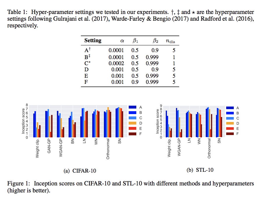
Adam optimizer: 6 settings in total, related to

• [math]\displaystyle{ n_{dis} }[/math], the number of updates of the discriminator per one update of Adam.
• learning rate [math]\displaystyle{ \alpha }[/math]
• the first and second momentum parameters [math]\displaystyle{ \beta_1, \beta_2 }[/math] of Adam

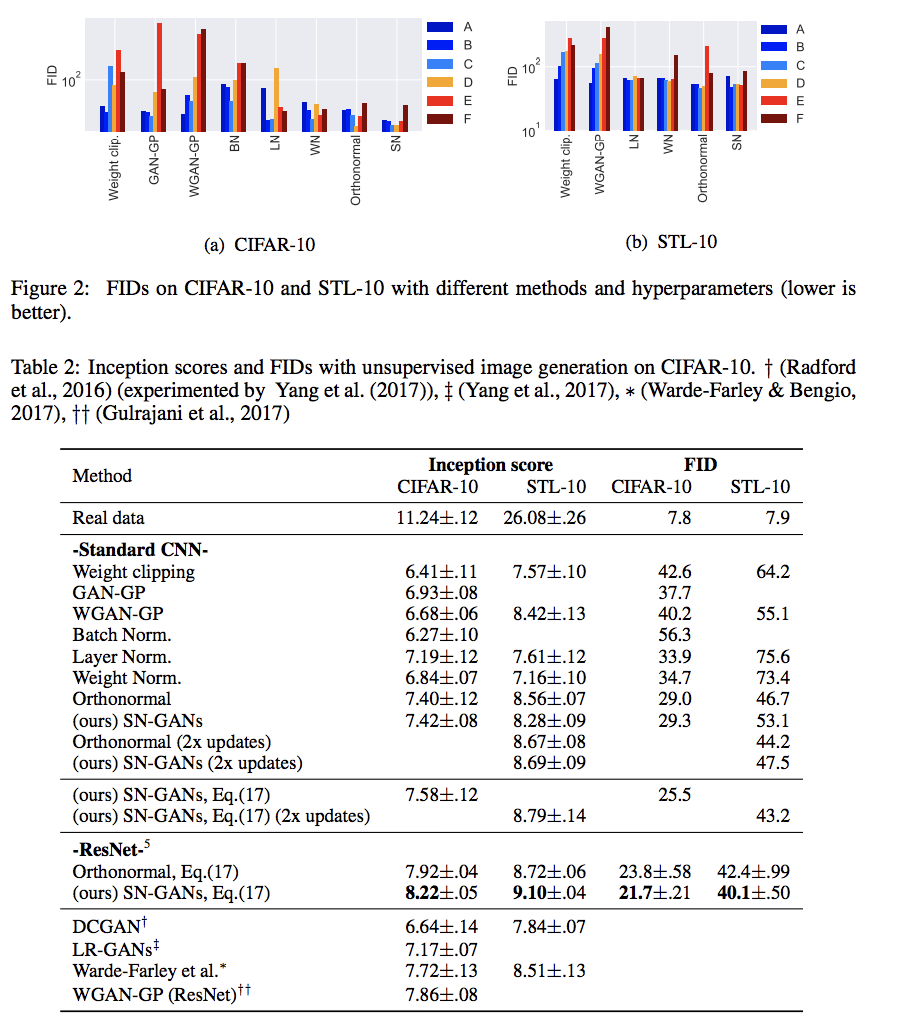
The above image show the inception core and FID score of with settings A-F, and table show the inception scores of the different methods with optimal settings on CIFAR-10 and STL-10 dataset.

Singular values analysis on the weights of the discriminator D

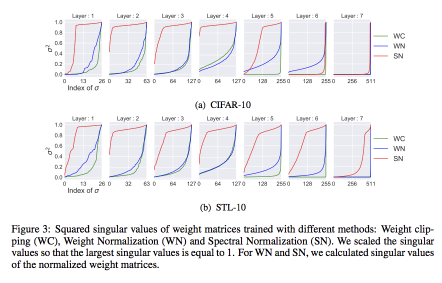
In above figure, we show the squared singular values of the weight matrices in the final discriminator D produced by each method using the parameter that yielded the best inception score. As we predicted before, the singular values of the first fifth layers trained with weight clipping and weight normalization concentrate on a few components. On the other hand, the singular values of the weight matrices in those layers trained with spectral normalization is more broadly distributed.

Training time

On CIFAR-10, SN-GANs is slightly slower than weight normalization, but significantly faster than WGAN-GP. As we mentioned in Section3, WGAN-GP is slower than other methods because WGAN-GP needs to calculate the gradient of gradient norm.

comparison between GN-GANs and orthonormal regularization

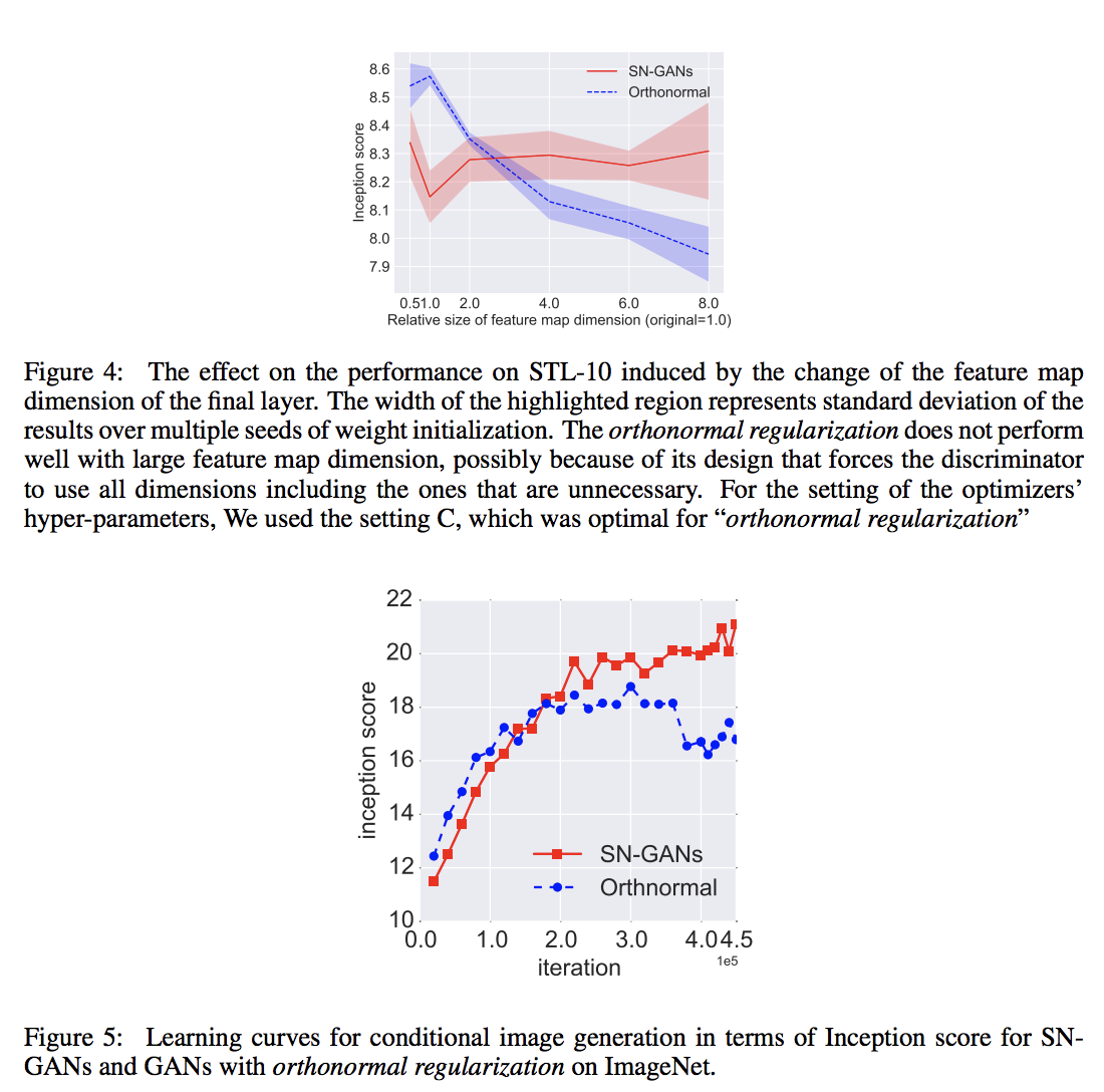
Above we explained in Section 3, orthonormal regularization is different from our method in that it destroys the spectral information and puts equal emphasis on all feature dimensions, including the ones that shall be weeded out in the training process. To see the extent of its possibly detrimental effect, we experimented by increasing the dimension of the feature space, especially at the final layer for which the training with our spectral normalization prefers relatively small feature space. Above figure shows the result of our experiments. As we predicted, the performance of the orthonormal regularization deteriorates as we increase the dimension of the feature maps at the final layer. SN-GANs, on the other hand, does not falter with this modification of the architecture.

We also applied our method to the training of class conditional GANs on ILSVRC2012 dataset with 1000 classes, each consisting of approximately 1300 images, which we compressed to 128*128 pixels. GAN without normalization and GAN with layer normalization collapsed in the beginning of training and failed to produce any meaningful images. Above picture shows that the inception score of the orthonormal normalization plateaued around 20k iterations, while SN kept improving even afterward.

Algorithm of spectral normalization

To calculate the largest singular value of matrix [math]\displaystyle{ W }[/math] to implement spectral normalization, we appeal to power iterations. Algorithm is executed as follows:

• Initialize [math]\displaystyle{ \tilde{u}_{l}\in R^{d_l} \text{for} l=1,\cdots,L }[/math] with a random vector (sampled from isotropic distribution)
• For each update and each layer l:
• Apply power iteration method to a unnormalized weight [math]\displaystyle{ W^l }[/math]:

[math]\displaystyle{ \tilde{v_l}\leftarrow (W^l)^T\tilde{u_l}/||(W^l)^T\tilde{u_l}||_2 }[/math]

[math]\displaystyle{ \tilde{u_l}\leftarrow (W^l)^T\tilde{v_l}/||(W^l)^T\tilde{v_l}|| }[/math]

• Calculate [math]\displaystyle{ \bar{W_{SN}} }[/math] with the spectral norm :

[math]\displaystyle{ \bar{W_{SN}}(W^l)=W^l/\sigma(W^l), \text{where} \sigma(W^l)=\tilde{u_l}^TW^l\tilde{v_l} }[/math]

• Update [math]\displaystyle{ W^l }[/math] with SGD on mini-batch dataset [math]\displaystyle{ D_M }[/math] with a learning rate [math]\displaystyle{ \alpha }[/math]

[math]\displaystyle{ W^l\leftarrow W^l-\alpha\nabla_{W^l}l(\bar{W_{SN}^l}(W^l),D_M) }[/math]

Conclusions

This paper proposes spectral normalization as a stabilizer of training of GANs. When we apply spectral normalization to the GANs on image generation tasks, the generated examples are more diverse than the conventional weight normalization and achieve better or comparative inception scores relative to previous studies. The method imposes global regularization on the discriminator as opposed to local regularization introduced by WGAN-GP, and can possibly used in combinations. In the future work, we would like to further investigate where our methods stand amongest other methods on more theoretical basis, and experiment our algorithm on larger and more complex datasets.