Word translation without parallel data

Presented by

Xia Fan

Introduction

This paper introduce a model that either is on par, or outperforms supervised state-of-the-art methods, without employing any cross-lingual annotated data. This method use a similar idea with GAN: it leverages adversarial training to learn a linear mapping from a source to a distinguish between the mapped source embeddings and the target embeddings, while the mapping is jointly trained to fool the discriminator. Second, this paper extract a synthetic dictionary from the resulting shared embedding space and fine-tune the mapping with the closed-form Procrustes solution from Schonemann (1966). Third, this paper also introduce an unsupervised selection metric that is highly correlated with the mapping quality and that we use both as a stopping criterion and to select the best hyper-parameters.

Model

Estimation of Word Representations in Vector Space

This model focuses on learning a mapping between the two sets such that translations are close in the shared space. Before talking about the model it used, a model which can exploit the similarities of monolingual embedding spaces should be introduced. Mikolov et al.(2013) use a known dictionary of n=5000 pairs of words [math]\displaystyle{ \{x_i,y_i\}_{i\in{1,n}} }[/math]. and learn a linear mapping W between the source and the target space such that

\begin{align} W^*=argmin_{W{\in}M_d(R)}||WX-Y||_F \hspace{1cm} (1) \end{align}

where d is the dimension of the embeddings, [math]\displaystyle{ M_d(R) }[/math] is the space of d*d matrices of real numbers, and X and Y are two aligned matrices of size d*n containing the embeddings of the words in the parallel vocabulary.

Xing et al. (2015) showed that these results are improved by enforcing orthogonality constraint on W. In that case, the equation (1) boils down to the Procrustes problem, which advantageously offers a closed form solution obtained from the singular value decomposition (SVD) of [math]\displaystyle{ YX^T }[/math] :

\begin{align} W^*=argmin_{W{\in}M_d(R)}||WX-Y||_F=UV^T, with U\Sigma V^T=SVD(YX^T) \end{align}

Domain-adversarial setting

This paper shows how to learn this mapping W without cross-lingual supervision. An illustration of the approach is given in Fig. 1. First, this model learn an initial proxy of W by using an adversarial criterion. Then, it use the words that match the best as anchor points for Procrustes. Finally, it improve performance over less frequent words by changing the metric of the space, which leads to spread more of those points in dense region.

Figure 1: Toy illustration of the method. (A) There are two distributions of word embeddings, English words in red denoted by X and Italian words in blue denoted by Y , which we want to align/translate. Each dot represents a word in that space. The size of the dot is proportional to the frequency of the words in the training corpus of that language. (B) Using adversarial learning, we learn a rotation matrix W which roughly aligns the two distributions. The green stars are randomly selected words that are fed to the discriminator to determine whether the two word embeddings come from the same distribution. (C) The mapping W is further refined via Procrustes. This method uses frequent words aligned by the previous step as anchor points, and minimizes an energy function that corresponds to a spring system between anchor points. The refined mapping is then used to map all words in the dictionary. (D) Finally, we translate by using the mapping W and a distance metric, dubbed CSLS, that expands the space where there is high density of points (like the area around the word “cat”), so that “hubs” (like the word “cat”) become less close to other word vectors than they would otherwise (compare to the same region in panel (A)).

Let [math]\displaystyle{ X={x_1,...,x_n} }[/math] and [math]\displaystyle{ Y={y_1,...,y_m} }[/math] be two sets of n and m word embeddings coming from a source and a target language respectively. A model is trained is trained to discriminate between elements randomly sampled from [math]\displaystyle{ WX={Wx_1,...,Wx_n} }[/math] and Y, We call this model the discriminator. W is trained to prevent the discriminator from making accurate predictions. As a result, this is a two-player game, where the discriminator aims at maximizing its ability to identify the origin of an embedding, and W aims at preventing the discriminator from doing so by making WX and Y as similar as possible. This approach is in line with the work of Ganin et al.(2016), who proposed to learn latent representations invariant to the input domain, where in our case, a domain is represented by a language(source or target).

1. Discriminator objective

Refer to the discriminator parameters as [math]\displaystyle{ \theta_D }[/math]. Consider the probability [math]\displaystyle{ P_{\theta_D}(source = 1|z) }[/math] that a vector z is the mapping of a source embedding (as opposed to a target embedding) according to the discriminator. The discriminator loss can be written as:

\begin{align} L_D(\theta_D|W)=-\frac{1}{n} \sum_{i=1}^n log P_{\theta_D}(source=1|Wx_i)-\frac{1}{m} \sum_{i=1}^m log P_{\theta_D}(source=0|Wx_i) \end{align}

2. Mapping objective

In the unsupervised setting, W is now trained so that the discriminator is unable to accurately predict the embedding origins:

\begin{align} L_W(W|\theta_D)=-\frac{1}{n} \sum_{i=1}^n log P_{\theta_D}(source=0|Wx_i)-\frac{1}{m} \sum_{i=1}^m log P_{\theta_D}(source=1|Wx_i) \end{align}

3. Learning algorithm To train our model, we follow the standard training procedure of deep adversarial networks of Goodfellow et al. (2014). For every input sample, the discriminator and the mapping matrix W are trained successively with stochastic gradient updates to respectively minimize [math]\displaystyle{ L_D }[/math] and [math]\displaystyle{ L_W }[/math]

Refinement procedre

The matrix W obtained with adversarial training gives good performance (see Table 1), but the results are still not on par with the supervised approach. In fact, the adversarial approach tries to align all words irrespective of their frequencies. However, rare words have embeddings that are less updated and are more likely to appear in different contexts in each corpus, which makes them harder to align. Under the assumption that the mapping is linear, it is then better to infer the global mapping using only the most frequent words as anchors. Besides, the accuracy on the most frequent word pairs is high after adversarial training. To refine our mapping, this paper build a synthetic parallel vocabulary using the W just learned with ad- versarial training. Specifically, this paper consider the most frequent words and retain only mutual nearest neighbors to ensure a high-quality dictionary. Subsequently, this paper apply the Procrustes solution in (2) on this generated dictionary. Considering the improved solution generated with the Procrustes al- gorithm, it is possible to generate a more accurate dictionary and apply this method iteratively, similarly to Artetxe et al. (2017). However, given that the synthetic dictionary obtained using ad- versarial training is already strong, this paper only observe small improvements when doing more than one iteration, i.e., the improvements on the word translation task are usually below 1%.

Cross-Domain similarity local scaling

In this paper, it considers a bi-partite neighborhood graph, in which each word of a given dictionary is connected to its K nearest neighbors in the other language. [math]\displaystyle{ N_T(Wx_s) }[/math] is used to denote the neighborhood, on this bi-partite graph, associated with a mapped source word embedding [math]\displaystyle{ Wx_s }[/math]. All K elements of [math]\displaystyle{ N_T(Wx_s) }[/math] are words from the target language. Similarly we denote by [math]\displaystyle{ N_S(y_t) }[/math] the neighborhood associated with a word t of the target language. Consider the mean similarity of a source embedding [math]\displaystyle{ x_s }[/math] to its target neighborhood as

\begin{align} r_T(Wx_s)=\frac{1}{K}\sum_{y\in N_T(Wx_s)}cos(Wx_s,y_t) \end{align}

where cos(,) is the cosine similarity. This is used to define similarity measure CSLS(.,.) between mapped source words and target words,as

\begin{align} CSLS(Wx_s,y_t)=2cos(Wx_s,y_t)-r_T(Wx_s)-r_S(y_t) \end{align}

Training and architectural choices

Architecture

This paper use unsupervised word vectors that were trained using fastText2. These correspond to monolin- gual embeddings of dimension 300 trained on Wikipedia corpora; therefore, the mapping W has size 300 × 300. Words are lower-cased, and those that appear less than 5 times are discarded for training. As a post-processing step, only the first 200k most frequent words were selected in the experiments. For the discriminator, it use a multilayer perceptron with two hidden layers of size 2048, and Leaky-ReLU activation functions. The input to the discriminator is corrupted with dropout noise with a rate of 0.1. As suggested by Goodfellow (2016), a smoothing coefficient s = 0.2 is included in the discriminator predictions. This paper use stochastic gradient descent with a batch size of 32, a learning rate of 0.1 and a decay of 0.95 both for the discriminator and W .

Discriminator inputs

The embedding quality of rare words is generally not as good as the one of frequent words (Luong et al., 2013), and it is observed that feeding the discriminator with rare words had a small, but not negligible negative impact. As a result, this paper only feed the discriminator with the 50,000 most frequent words. At each training step, the word embeddings given to the discriminator are sampled uniformly. Sampling them according to the word frequency did not have any noticeable impact on the results.

Orthogonality

In this work, it propose to use a simple update step to ensure that the matrix W stays close to an orthogonal matrix during training (Cisse et al. (2017)). Specifically, the following update rule on the matrix W is used :

\begin{align} W \leftarrow (1+\beta)W-\beta(WW^T)W \end{align}

where β = 0.01 is usually found to perform well. This method ensures that the matrix stays close to the manifold of orthogonal matrices after each update.

Dictionary generation

The refinement step requires to generate a new dictionary at each iteration. In order for the Procrustes solution to work well, it is best to apply it on correct word pairs. As a result, the CSLS method is used to select more accurate translation pairs in the dictionary. To increase even more the quality of the dictionary, and ensure that W is learned from correct translation pairs, only mutual nearest neighbors were considered, i.e. pairs of words that are mutually nearest neighbors of each other according to CSLS. This significantly decreases the size of the generated dictionary, but improves its accuracy, as well as the overall performance.

Validation criterion for unsupervised model selection

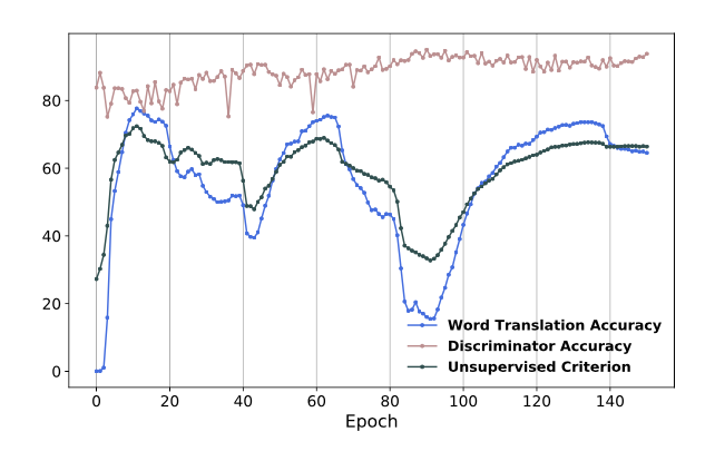
This paper consider the 10k most frequent source words, and use CSLS to generate a translation for each of them, then compute the average cosine similarity between these deemed translations, and use this average as a validation metric. Figure 2 shows the correlation between the evaluation score and this unsupervised criterion (without stabilization by learning rate shrinkage)

Figure 2: Unsupervised model selection. Correlation between our unsupervised vali- dation criterion (black line) and actual word translation accuracy (blue line). In this par- ticular experiment, the selected model is at epoch 10. Observe how our criterion is well correlated with translation accuracy.

Results

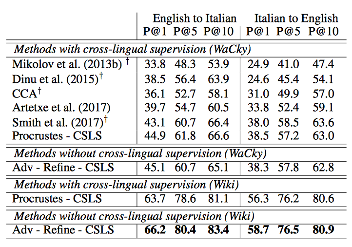
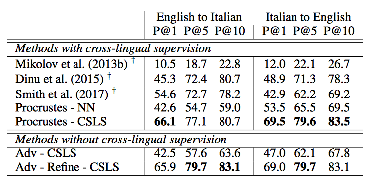
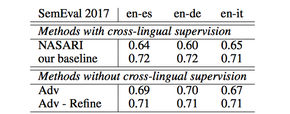
In what follows, the results on word translation retrieval using our bilingual dictionaries were presented in Table 1 and the comparison to previous work in Table 2 where unsupervised model significantly outperform previous approaches. The results on the sentence translation retrieval task were also presented in Table 3 and the cross-lingual word similarity task in Table 4. Finally, the results on word-by-word translation for English-Esperanto was presented in Table 5.

Table 1: Word translation retrieval P@1 for our released vocabularies in various language pairs. We consider 1,500 source test queries, and 200k target words for each language pair. We use fastText embeddings trained on Wikipedia. NN: nearest neighbors. ISF: inverted softmax. (’en’ is English, ’fr’ is French, ’de’ is German, ’ru’ is Russian, ’zh’ is classical Chinese and ’eo’ is Esperanto)

English-Italian word translation average precisions (@1, @5, @10) from 1.5k source word queries using 200k target words. Re- sults marked with the symbol † are from Smith et al. (2017). Wiki means the embeddings were trained on Wikipedia using fastText. Note that the method used by Artetxe et al. (2017) does not use the same super- vision as other supervised methods, as they only use numbers in their ini- tial parallel dictionary.

Table 3: English-Italian sentence translation retrieval. We report the average P@k from 2,000 source queries using 200,000 target sen- tences. We use the same embeddings as in Smith et al. (2017). Their re- sults are marked with the symbol †.

Table 4: Cross-lingual wordsim task. NASARI (Camacho-Collados et al. (2016)) refers to the official SemEval2017 baseline. We report Pearson correlation.

Table 5: BLEU score on English-Esperanto. Although being a naive approach, word-by- word translation is enough to get a rough idea of the input sentence. The quality of the gener- ated dictionary has a significant impact on the BLEU score.

Criticisms

There is some concern regarding whether this model will be able to provide a truly scalable solution to MT. In particular, it is not obvious that this model will be able to sufficiently scale to long sentences as is evident in the reported results. The model is severely limited, in general, by working only in the absence of infrequent words. These theoretical limitations alongside sparse experimental results give rise to skepticism about the overarching validity of the model.

Source

Sutskever, I. Vinyals, O. & Le. Q. V. Sequence to sequence learning with neural networks. In Proc. Advances in Neural Information Processing Systems 27 3104–3112 (2014). <references />