STAT946F17/ Automated Curriculum Learning for Neural Networks
Introduction
Humans and animals learn much better when the examples are not randomly presented but organized in a meaningful order which illustrates gradually more concepts, and gradually more complex ones. Here, we formalize such training strategies in the context of machine learning, and call them “curriculum learning”. The idea of training a learning machine with a curriculum can be traced back at least to Elman (1993). The basic idea is to start small, learn easier aspects of the task or easier sub-tasks, and then gradually increase the difficulty level.
However curriculum learning has only recently become prevalent in the field (e.g., Bengio et al., 2009), due in part to the greater complexity of problems now being considered. In particular, recent work on learning programs with neural networks has relied on curricula to scale up to longer or more complicated tasks (Reed and de Freitas, 2015, Gui et al. 2017). We expect this trend to continue as the scope of neural networks widens, with deep reinforcement learning providing fertile ground for structured learning.
One reason for the slow adoption of curriculum learning is that it’s effectiveness is highly sensitive to the mode of progression through the tasks. One popular approach is to define a hand-chosen performance threshold for advancement to the next task, along with a fixed probability of returning to earlier tasks, to prevent forgetting (Sutskever and Zaremba, 2014). However, as well as introducing hard-to-tune parameters, this poses problems for curricula where appropriate thresholds may be unknown or variable across tasks.
The main contribution of the paper is that a stochastic policy, continuously adapted to optimize learning progress is proposed. Given a progress signal that can be evaluated for each training example, we use a multi-armed bandit algorithm to find a stochastic policy over the tasks that maximizes overall progress. The bandit is non-stationary because the behaviour of the network, and hence the optimal policy, evolves during training. Moreover variants of prediction gain, and also a novel class of progress signals which we refer to as complexity gain are considered in this paper.
Model
A task is a distribution $D$ over sequences from $\mathcal{X}$ . A curriculum is an ensemble of tasks $D_1, \ldots D_N$ , a sample is an example drawn from one of the tasks of the curriculum, and a syllabus is a time-varying sequence of distributions over tasks. A neural network is considered as a probabilistic model $p_\theta$ over $\mathcal{X}$, whose parameters are denoted $\theta$.
The expected loss of the network on the $k$-th task is \[ \mathcal{L}_k( \theta) := \mathbb{E}_{\mathbf{x} \sim D_k} L(\mathbf{x}, \theta), \] where $L(\mathbf{x}, \theta):= -\log_{p_\theta}(\mathbf{x})$ is the sample loss on $\mathbf{x}$.
A curriculum containing $N$ tasks as an $N$-armed bandit, and a syllabus as an adaptive policy which seeks to maximize payoffs from this bandit. In the bandit setting, an agent selects a sequence of arms (actions) $a_1,\ldots, a_T$ over T rounds of play. After each round, the selected arm yields a payoff $r_t$; the payoffs for the other arms are not observed.
Adversarial Multi-Armed Bandits
The classic algorithm for adversarial bandits is Exp3, which minimize regret with respect to the single best arm evaluated over the whole history. However, in the case of training neural network, an arm is optimal for a portion of the history, then another arm, and so on; the best strategy is then piecewise stationary. The Fixed Share method addresses this issue by using an $\epsilon$-greedy strategy. It is known as the Exp3.S algorithm.
On round $t$, the agent selects an arm stochastically according to a policy $\pi_t$ . This policy is defined by a set of weights $w_t$, \[ \pi_t(i) := (1-\epsilon)\frac{e^{w_{t,i}}}{\sum_{j=1}^N e^{w_{t,j}}}+\frac{\epsilon}{N} \] \[ w_{t,i}:= \log \big[ (1-\alpha_t)\exp\{ w_{t-1,i} +\eta \bar{r}_{t-1,i}^\beta \} +\frac{\alpha_t}{N-1}\sum_{j \ne i} \exp\{ w_{t-1,j} +\eta \bar{r}_{t-1,j}^\beta \} \big] \] \[ w_{1,i} = 0, \quad \alpha_t = t^{-1} , \quad \bar{r}_{s,i}^\beta = \frac{r_s \mathbb{I}_{[a_s = i]}+ \beta}{ \pi_s(i) } \]
Reward Scaling
The appropriate step size $\eta$ depends on the magnitudes of the rewards, which may not be known. The magnitude of reward depends strongly on the gain signal used to measure learning progress, as well as varying over time as the model learns. To address this issue, all rewards are adaptively rescale to $[-1,1]$ by \[ r_t = \begin{cases} -1 &\quad \text{if } \hat{r}_t < q^{l}_t\\ 1 &\quad \text{if } \hat{r}_t > q^{h}_t\\ \frac{2(\hat{r}_t-q^l_t)}{q^h_t-q^l_t} -1 , &\quad \text{otherwise.} \end{cases} \] where $q^l_t$ and $q^h_t$ are the quantiles of the history of unscaled rewards up to time $t$. The authors chose them to be $20$-th and $80$-th percentiles respectively.
Algorithm
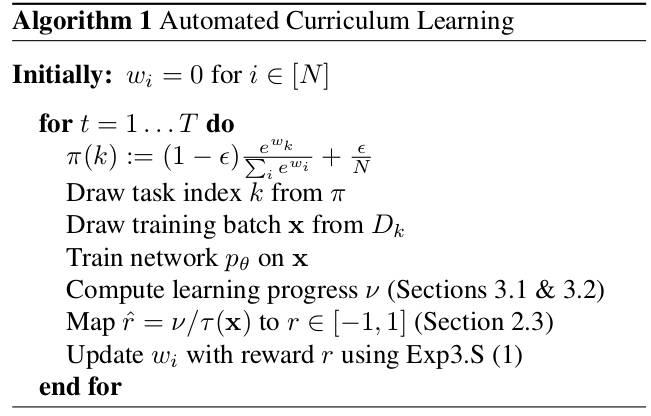
The automated curriculum learning is summarized as followed,
where $\tau(\mathbf{x})$ is the length of the longest input sequence. Since the processing time of each task may be different.
