STAT946F17/Conditional Image Generation with PixelCNN Decoders

Introduction

This works is based of the widely used PixelCNN and PixelRNN, introduced by Oord et al. in [1]. From the previous work, the authors observed that PixelRNN performed better than PixelCNN, however, PixelCNN was faster to compute as you can parallize the training process. In this work, Oord et al. [2] introduced a Gated PixelCNN, which is a convolutional variant of the PixelRNN model, based on PixelCNN. In particular, the Gated PixelCNN uses explicit probability densities to generate new images using autoregressive connections to model images through pixel-by-pixel computation by decomposing the joint image distribution as a product of conditionals. The Gated PixelCNN is an improvement over the PixelCNN by removing the "blindspot" problem, and to yield a better performance, the authors replaced the ReLU units with sigmoid and tanh activation function. The proposed Gated PixelCNN combines the strength of both PixelRNN and PixelCNN - that is by matching the log-likelihood of PixelRNN on both CIFAR and ImageNet along with the quicker computational time presented by the PixelCNN. Moreover, the authors also introduced a conditional Gated PixelCNN variant (called Conditional PixelCNN) which has the ability to generate images based on class labels, tags, as well as latent embeddings to create new image density models. These embeddings capture high level information of an image to generate a large variety of images with similar features; for instance, the authors can generate different poses of a person based on a single image by conditioning on a one-hot encoding of the class. This approach provided insight into the invariances of the embeddings which enabled the authors to generate different poses of the same person based on a single image. Finally, the authors also presented a PixelCNN Auto-encoder variant which essentially replaces the deconvolutional decoder with the PixelCNN.

Gated PixelCNN

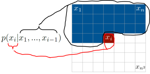
Pixel-by-pixel is a simple generative method wherein given an image of dimension of dimension $x_{n^2}$, we iterate, employ feedback and capture pixel densities from every pixel to predict our "unknown" pixel density $x_i$. To do this, the traditional PixelCNNs and PixelRNNs adopted the joint distribution p(x), wherein the pixels of a given image is the product of the conditional distributions. Hence, the authors employ autoregressive models which means they just use plain chain rule for joint distribution, depicted in Equation 1. So the very first pixel is independent, second depend on first, third depends on first and second and so on. Basically you just model your image as sequence of points where each pixel depends linearly on previous ones. Equation 1 depicts the joint distribution where x_i is a single pixel:

$$p(x) = \prod\limits_{i=1}^{n^2} p(x_i | x_1, ..., x_{i-1})$$

where $p(x)$ is the generated image, $n^2$ is the number of pixels, and $p(x_i | x_1, ..., x_{i-1})$ is the probability of the $i$th pixel which depends on the values of all previous pixels. It is important to note that $p(x_0, x_1, ..., x_{n^2})$ is the joint probability based on the chain rule - which is a product of all conditional distributions $p(x_0) \times p(x_1|x_0) \times p(x_2|x_1, x_0)$ and so on. Figure 1 provides a pictoral understanding of the joint distribution which displays that the pixels are computed pixel-by-pixel for every row, and the forthcoming pixel depends on the pixels values above and to the left of the pixel in concern.

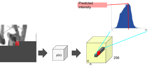
Hence, for every pixel, we use the softmax layer towards the end of the PixelCNN to predict the pixel intensity value (i.e. the highest probable index from 0 to 255). Figure 2 illustrates how to predict (generate) a single pixel value.

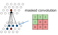
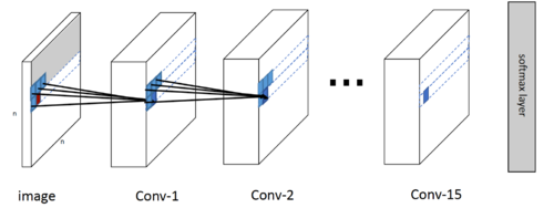
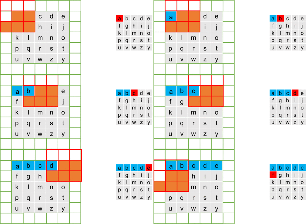
So, the PixelCNN is supposedly to maps a neighborhood of pixels to prediction for the next pixel. That is, to generate pixel $x_i$ the model can only condition on the previously generated pixels $x_1 , ..., x_{i−1}$; so every conditional distribution is modelled by a convolutional neural network. For instance, given a $5\times5$ image (let's represent each pixel as an alphabet and zero-padded), and we have a filter of dimension $3\times3$ that slides over the image which multiplies each element and sums them together to produce a single response. However, we cannot use this filter because pixel $a$ should not know the pixel intensities for $b,f,g$ (future pixel values). To counter this issue, the authors use a mask on top of the filter to only choose prior pixels and zeroing the future pixels to negate them from calculation - depicted in Figure 3. Hence, to make sure the CNN can only use information about pixels above and to the left of the current pixel, the filters of the convolution are masked - that means the model cannot read pixels below (or strictly to the right) of the current pixel to make its predictions - illustrated in Figure 4.

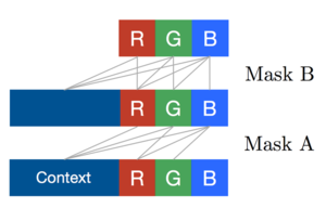
Hence, for each pixel there are three colour channels (R, G, B) which are modelled successively, with B conditioned on (R, G), and G conditioned on R. This is achieved by splitting the feature maps at every layer of the network into three and adjusting the centre values of the mask tensors, as depicted in Figure 5. The 256 possible values for each colour channel are then modelled using a softmax.

Figure 5: RGB Masking

Now, from Figure 6, notice that as the filter with the mask slides across the image, pixel $f$ does not take pixels $c, d, e$ into consideration (breaking the conditional dependency) - this is where we encounter the "blind spot" problem.

It is evident that the progressive growth of the receptive field of the masked kernel over the image disregards a significant portion of the image. For instance, when using a 3x3 filter, roughly quarter of the receptive field is covered by the "blind spot", meaning that the pixel contents are ignored in that region. In order to address the blind spot, the authors use two filters (horizontal and vertical stacks) in conjunction to allow for capturing the whole receptive field, depicted in Figure 7. In particular, the horizontal stack conditions the current row, and the vertical stack conditions all the rows above the current pixel. It is observed that the vertical stack, which does not have any masking, allows the receptive field to grow in a rectangular fashion without any blind spot. Thereafter, the outputs of both the stacks, per-layer, is combined to form the output. Hence, every layer in the horizontal stack takes an input which is the output of the previous layer as well as that of the vertical stack. By spliting the convolution into two different operations enables the model to access all pixels prior to the pixel of interest.

Summary

$\bullet$ Improved PixelCNN

1. Similar performance as PixelRNN, and quick to compute like PixelCNN (since it is easier to parallelize)
2. Fixed the "blind spot" problem by introducing 2 stacks (horizontal and vertical)
3. Gated activation units which now use sigmoid and tanh instead of ReLU units

$\bullet$ Conditioned Image Generation

1. One-shot conditioned on class-label
2. Conditioned on portrait embedding
3. Pixel AutoEncoders

Reference

1. Aaron van den Oord et al., "Pixel Recurrent Neural Network", ICML 2016
2. Aaron van den Oord et al., "Conditional Image Generation with PixelCNN Decoders", NIPS 2016