Universal Style Transfer via Feature Transforms
Introduction
When viewing an image, whether it is a photograph or a painting, two types of mutually exclusive data are present. First, there is the content of the image, such as a person in a portrait. However, the content does not uniquely define the image. Consider a case where multiple artists paint a portrait of an identical subject, the results would vary despite the content being invariant. The cause of the variance is rooted in the style of each particular artist. Therefore, style transfer between two images results in the content being unaffected but the style being copied. Typically one image is termed the content/reference image, whose style is discarded. The other image is called the style image, whose style, but not content is copied to the content image.
Deep learning techniques have been shown to be effective methods for implementing style transfer. Previous methods have been successful but with several key limitations. Either they are fast, but have very few styles that can be transferred or they can handle arbitrary styles but are no longer efficient. The presented paper establishes a compromise between these two extremes by using only whitening and colouring transforms (WCT) to transfer a style. No training of the underlying deep network is required per style.
Related Work
Gatys et al. developed a new method for generating textures from sample images in 2015 [1] and extended their approach to style transfer by 2016 [2]. They proposed the use of a pre-trained convolutional neural network (CNN) to separate content and style of input images. Having proven successful, a number of improvements quickly developed, reducing computational time, increasing the diversity of transferrable styes, and improving the quality of the results. Central to these approaches and of the present paper is the use of a CNN.
How Content and Style are Extracted using CNNs
A CNN was chosen due to its ability to extract high level features from images. These features can be interpreted in two ways. Within layer [math]\displaystyle{ l }[/math] there are [math]\displaystyle{ N_l }[/math] features maps of size [math]\displaystyle{ M_l }[/math]. With a particular input image, the feature maps are given by [math]\displaystyle{ F_{i,j}^l }[/math] where [math]\displaystyle{ i }[/math] and [math]\displaystyle{ j }[/math] locate the map within the layer. Starting with a white noise image and an reference (content) image, the features can be transferred by minimizing
[math]\displaystyle{ \mathcal{L}_{content} = \frac{1}{2} \sum_{i,j} \left( F_{i,j}^l - P_{i,j}^l \right)^2 }[/math]
where [math]\displaystyle{ P_{i,j} }[/math] denotes the feature map output caused by the white noise image. Therefore this loss function preserves the content of the reference image. The style is described using a Gram matrix given by
[math]\displaystyle{ G_{i,j}^l = \sum_k F_{i,k}^l F_{j,k}^l }[/math]
and the loss function that describes a difference in style between two images is
[math]\displaystyle{ \mathcal{L}_{style} = \frac{1}{4 N_l^2 M_l^2} \sum_{i,j} \left(G_{i,j}^l - A_{i,j}^l \right)^2 }[/math]
where [math]\displaystyle{ A_{i,j}^l }[/math] and [math]\displaystyle{ G_{i,j}^l }[/math] are the Gram matrices of the generated image and style image respectively. Therefore three images are required, a style image, a content image and an initial white noise image. Iterative optimization is then used to add content from one image to the white noise image, and style from the other. An additional parameter is used to balance the ratio of these loss functions.
The 19-layer ImageNet trained VGG network was chosen by Gatys et al. VGG-19 is still commonly used in more recent works as will be shown in the presented paper, although training datasets vary. Such CNNs are typically used in classification problems by finalizing their output through a series of full connected layers. For content and style extraction it is the convolutional layers that are required. The method of Gatys et al. is style independent, since the CNN does not need to be trained for each style image. However the process of iterative optimization to generate the output image is computational expensive.
Other Methods
Other methods avoid the inefficiency of iterative optimization by training a network/networks on a set of styles. The network then directly transfers the style from the style image to the content image without solving the interative optimization problem. V. Dumoulin et al. trained a single network on $N$ styles [3]. This improved upon previous work where a network was required per style [4]. The stylized output image was generated by simply running a feedforward pass of the network on the content image. While efficiency is high, the method is no longer able to apply an arbitrary style without retraining.
Methodology
Li et al. have proposed a novel method for generating the stylized image. A CNN is still used as in Gatys et al. to extract content and style. However, the stylized image is not generated through iterative optimization or a feed-forward pass as required by previous methods. Instead, whitening and colour transforms are used.
Image Reconstruction

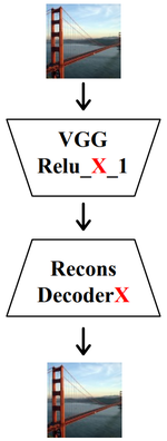
An auto-encoder network is used to first encode an input image into a set of feature maps, and then decode it back to an image as shown in the adjacent figure. The encoder network used is VGG-19. This network is reponsible for obtaining feature maps (similar to Gatys et al.). The output of each of the first five layers is then fed into a corresponding decoder network, which is a mirrored version of VGG-19. Each decoder network then decodes the feature maps of the $l$th layer producing an output image. A mechanism for transferring style will be implemented by manipulating the feature maps between the encoder and decoder networks.
First, the auto-encoder network needs to be trained. The following loss function is used
[math]\displaystyle{ \mathcal{L} = || I_{output} - I_{input} ||_2^2 + \lambda || \Phi(I_{output}) - \Phi(I_{input})||_2^2 }[/math]
where $I_{input}$ and $I_{output}$ are the input and output images of the auto-encoder. $\Phi$ is the VGG encoder. The first term of the loss is the pixel reconstruction loss, while the second term is feature loss. Recall from "Related Work" that the feature maps correspond to the content of the image. Therefore the second term can also be seen as penalising for content differences that arise due to the encoder network. The network was trained using the Microsoft COCO dataset.
Whitening Transform
Whitening first requires that the covariance of the data is a diagonal matrix. This is done by solving for the covariance matrix's eigenvalues and eigenvector matrices. Whitening then forces the diagonal elements of the eigenvalue matrix to be the same. This is achieved for a feature map from VGG through the following steps.
- The feature map $f_c$ is extracted from a layer of the encoder network after activation on the content image. This is the data to be whitened.
- $f_c$ is centered by subtracting its mean vector $m_c$.
- Then, the eigenvectors $E_c$ and eigenvalues $D_c$ are found for the covariance matrix of $f_c$.
- The whitened feature map is then given by $\hat{f}_c = E_c D_c^{-1/2} E_c^T f_c$.
If interested, the derivation of the whitening equation can be seen in [5]. Li et al. found that whitening removed styles from the image.
Colour Transform
However, whitening does not transfer style from the style image. It only uses feature maps from the content image. The colour transform uses both $\hat{f}_c$ from above and $f_s$, the feature map from the style image.
- $f_s$ is centered by subtracting its mean vector $m_s$.
- Then, the eigenvectors $E_s$ and eigenvalues $D_s$ are calculated for the covariance matrix of $f_s$.
- The colour transform is given by $\hat{f}_{cs} = E_s D_s^{1/2} E_s^T \hat{f}_c$.
- Recenter $\hat{f}_{cs}$ using $m_s$.
Intuitively, colouring results in a correlation between the $\hat{f}_c$ and $f_s$ feature maps. This is where the style transfer takes place.
Content/Style Balance
Using just $\hat{f}_{cs}$ as the input to the decoder may create a result that is too extreme in style. To balance content and style a new parameter $\alpha$ is defined.
[math]\displaystyle{ \hat{f}_{cs} = \alpha \hat{f}_{cs} + (1 - \alpha) f_c }[/math]
Using Multiple Layers
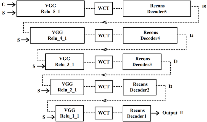
It has been previously mentioned that multiple decoders were trained, one for each of the first five layers of the encoder network. Each layer of a CNN perceives features at different levels. Levels close to the input image will detect lower level local features such as edges. Those levels deeper into the network will detect more complex global features. The style transfer algorithm is applied at each of these levels, which yields the question as to which results, as shown below, to use.

Ideally, the results of each layer should be used to build the final output image. This captures the entire range of features detected by the encoder network. First, one full pass of the network is performed. Then the stylised image from the deepest layer (Relu_5_1 in this case) is taken and used as the content image for another iteration of the algorithm, where then the next layer (Relu_4_1) is used as the output. These steps are repeated until the final image is produced from the shallowest layer. This process is summarised in the figure below.

Evaluation
The success of style transfer might appear hard to quantify as it relies on qualitative judgement. However the extremes of transferring no style, or transferring only style can be considered as performing poorly. Consistent transfer of style throughout the entire image is another parameter of success. Ideally, the viewer can recognize the content of the image, while seeing it expressed in an alternative style. Quantitatively, the quality of the style transfer can be calculated by taking the covariance matrix difference $L_s$ between the resulting image and the original style. The results of the presented paper also need to be considered within the contexts of generality, efficiency and training requirements.
Style Transfer
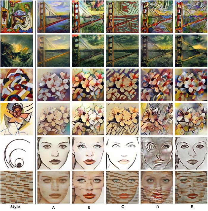
A number of style transfer examples are presented relative to other works.

Li et al. then obtained the average $L_s$ using 10 random content images across 40 style images. They had the lowest average $log(L_s)$ of all referenced works at 6.3. Next lowest was Gatys et al. [2] with $log(L_s) = 6.7$. It should be noted that while $L_s$ quantitatively calculates the success of the style transfer, results are still subject to the viewer's impression. Reviewing the transfer results, rows five and six for Gatys et al.'s method shows local minimization issues. However, their method still achieves a competitive $L_s$ score.
Transfer Efficiency
It was hypothesized by Li et al. that using WCT would enable faster run-times than [2] while still supporting arbitrary style transfer. For a 256x256 image, using a 12GB TITAN X, they achieved a transfer time of 1.5 seconds. Gatys et al.'s method [2] required 21.2 seconds. The pure feed forward approaches [7], and [8] had times equal to or less than 0.2 seconds. [6] had a time comparable to the presented paper's method. However, [6,7,8] do not generalize well to multiple styles as training is required. Therefore this paper obtained a near 15x speed up for a style agnostic transfer algorithm when compared to leading previous work. The authors also note that WCT was done using the CPU. They intend to port WCT to the GPU and expect to see the computational time be further reduced.
Other Applications
Li et al.'s method can also be used for texture synthesis. This was the original work of Gatys et. al. before they applied their algorithm to style transfer problems. Texture synthesis takes a reference texture/image and creates new textures from it. With proper boundary conditions enforced these synthesized textures can be tilable. Alternatively, higher resolution textures can be generated. Texture synthesis has applications in areas such as computer graphics, allowing for large surfaces to be texture mapped.
The content image is set as white noise, similar to how [2] initializes their output image. Then the reference texture/image is set as the style image. Since the content image is initially random white noise, then the features generated by the encoder of this image are also random. Li et al. state that this increases the diversity of the resulting output textures.

Reviewing the examples from the above figure, it can be observed that the method from this paper repeats fewer local features from the image than a competing feed forward network method [8]. While the analysis is qualitative, the authors claim that their method produces "more visually pleasing results".
Conclusion
Only a couple years ago were CNNs first used to stylize images. Today, a host of improvements have been developed, optimizing the original work of Gatys et al. for a number of different situations. Using additional training per style image, computational efficiency and image quality can be increased. However, the trained network then depends on that specific style image, or in some cases such as in [3], a set of style images. Till now, limited work has taken place in improving Gatys et al.'s method for arbitrary style images. The authors of this paper developed and evaluated a novel method for arbitrary style transfer. Their method and Gatys et al.'s method share the use of a VGG-19 CNN as the initial processing step. However, the authors replaced iterative optimization with whitening and colour transforms, which can be applied in a single step. This yields a decrease in computational time while maintaining generality with respect to the style image. After their CNN auto-encoder is initially trained no further training is required. This allows their method to be style agnostic. Their method also performs favourably, in terms of image quality, when compared to other current work.
Critique
In the paper, the authors only experimented with layers of VGG19. Given that architectures such as ResNet and Xception perform better on image recognition tasks, it would be interesting to see how residual layers and/or Inception modules may be applied to the task of disentangling style and content and whether they would improve performance relative to the results presented in the current paper is the encoder used were to utilize layers from these alternative convolutional architectures. Additionally, it is worth exploring whether one can invent a probabilistic and/or generative version of the encoder-decoder architecture used in the paper. More precisely, is it possible to come up with something in the spirit of variational autoencoders, wherein we the bottleneck layer can be used to sample noise vectors, which can then be input into each of the decoder units to generate synthetic style and content images.
References
[1] L. A. Gatys, A. S. Ecker, and M. Bethge. Texture synthesis using convolutional neural networks. In NIPS, 2015.
[2] L. A. Gatys, A. S. Ecker, and M. Bethge. Image style transfer using convolutional neural networks. In CVPR, 2016.
[3] V. Dumoulin, J. Shlens, and M. Kudlur. A learned representation for artistic style. In ICLR, 2017.
[4] J. Johnson, A. Alahi, and L. Fei-Fei. Perceptual losses for real-time style transfer and super-resolution. In ECCV, 2016
[5] R. Picard. MAS 622J/1.126J: Pattern Recognition and Analysis, Lecture 4. http://courses.media.mit.edu/2010fall/mas622j/whiten.pdf
[6] T. Q. Chen and M. Schmidt. Fast patch-based style transfer of arbitrary style. arXiv preprint arXiv:1612.04337, 2016.
[7] X. Huang and S. Belongie. Arbitrary style transfer in real-time with adaptive instance normalization. arXiv preprint arXiv:1703.06868, 2017.
[8] D. Ulyanov, V. Lebedev, A. Vedaldi, and V. Lempitsky. Texture networks: Feed-forward synthesis of textures and stylized images. In ICML, 2016.
[9] Leon A. Gatys, Alexander S. Ecker, Matthias Bethge, A Neural Algorithm of Artistic Style, https://arxiv.org/abs/1508.06576
[10] Karen Simonyan et al. Very Deep Convolutional Networks for Large-Scale Image Recognition
[11] VGG Architectures - More Details
Implementation Example: https://github.com/titu1994/Neural-Style-Transfer