very Deep Convoloutional Networks for Large-Scale Image Recognition

Introduction

In this paper<ref> Simonyan, Karen, and Andrew Zisserman. "Very deep convolutional networks for large-scale image recognition." arXiv preprint arXiv:1409.1556 (2014).</ref> the effect of the convolutional network depth on its accuracy in the large-scale image recognition setting is investigated. It was demonstrated that the representation depth is beneficial for the classification accuracy and the main contribution is a thorough evaluation of networks of increasing depth using a certain architecture with very small (3×3) convolution filters. Basically, they fix other parameters of the architecture, and steadily increase the depth of the network by adding more convolutional layers, which is feasible due to the use of very small (3 × 3) convolution filters in all layers. As a result, they come up with significantly more accurate ConvNet architectures.

Conv.Net Configurations

Architecture:

During training, the only preprocessing step is to subtract the mean RBG value computed on the training data. Then, the image is passed through a stack of convolutional (conv.) layers with filters with a very small receptive field: 3 × 3 with a convolutional stride of 1 pixel. Spatial pooling is carried out by five max-pooling layers, which follow some of the conv. Layers. Max-pooling is performed over a 2 × 2 pixel window, with stride 2. A stack of convolutional layers (which has a different depth in different architectures) is followed by three Fully-Connected (FC) layers. The final layer is the soft-max layer and all hidden layers are equipped with the rectification non-linearity.

They don't implement Local Response Normalization (LRN) as they found such normalization does not improve the performance on the ILSVRC dataset, but leads to increased memory consumption and computation time.

Configuration:

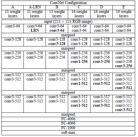
The ConvNet configurations, evaluated in this paper, are outlined in the following table:

All configurations follow the aforementioned architecture and differ only in the depth from 11 weight layers in the network A (8 conv. and 3 FC layers) to 19 weight layers in the network E (16 conv. and 3 FC layers) (the added layers are shown in bold). Besides, the width of conv. layers (the number of channels) is rather small, starting from 64 in the first layer and then increasing by a factor of 2 after each max-pooling layer, until it reaches 512.

As stated in the table, multiple convolutional layers with small filters are used without any maxpooling layer between them. It is easy to show that a stack of two 3×3 conv. layers (without spatial pooling in between) has an effective receptive field of 5×5, but using two/three stack of conv. layers have 2 main advantages: 1) Two/three non-linear rectification layers are incorporated instead of a single one, which makes the decision function more discriminative. 2) the number of parameters is decreased.

In the meantime, Since the 1×1 convolution is essentially a linear projection onto the space of the same dimensionality, the incorporation of 1 × 1 conv. layers (configuration C) is a way to increase the nonlinearity of the decision function without affecting the receptive fields of the conv. layers because of the rectification function.

Classification Framework

In this section, the details of classification ConvNet training and evaluation is described.

Training

Training is carried out by optimizing the multinomial logistic regression objective using mini-batch gradient descent with momentum. Initial weights for some layers were obtained from configuration “A” which is shallow enough to be trained with random initialization. The intermediate layers in deep models were initialized randomly. In spite of the larger number of parameters and the greater depth of the introduced nets, these nets required relatively fewer epochs to converge due to the following reasons: (a) implicit regularization imposed by greater depth and smaller conv. filter sizes. (b) using pre-initialization of certain layers.

With respect to (b) above, the shallowest configuration (A in the previous table) was trained using random initialization. For all the other configurations, the first four convolutional layers and the last 3 fully connected layers were initialized with the corresponding parameters from A, to avoid getting stuck during training due to a bad initialization. All other layers were randomly initialized by sampling from a normal distribution with 0 mean. The author also mentioned that they find it is possible to o initialise the weights without pre-training by using the random initialisation procedure of Glorot & Bengio<ref> Glorot, Xavier, and Yoshua Bengio. "Understanding the difficulty of training deep feedforward neural networks." International conference on artificial intelligence and statistics. 2010. </ref>

During training, the input to the ConvNets is a fixed-size 224 × 224 RGB image. To obtain this fixed-size image, rescaling has been done while training (one crop per image per SGD iteration). In order to rescale the input image, a training scale, from which the ConvNet input is cropped, should be determined. Two approaches for setting the training scale S (Let S be the smallest side of an isotropically-rescaled training image) is considered: 1) single-scale training, that requires a fixed S. 2) multi-scale training, where each training image is individually rescaled by randomly sampling S from a certain range [Smin, Smax] .

Implementation

To improve overall training speed of each model, the researchers introduced parallelization to the mini batch gradient descent process. Since the model is very deep, training on a single GPU would take months to finish. To speed up the process, the researchers trained separate batches of images on each GPU in parallel to calculate the gradients. For example, with 4 GPUs, the model would take 4 batches of images, calculate their separate gradients and then finally take an average of four sets of gradients as training. (Krizhevsky et al., 2012) introduced more complicated ways to parallelize training convolutional neural networks but the researchers found that this simple configuration speed up training process by a factor of 3.75 with 4 GPUs and with a possible maximum of 4, the simple configuration worked well enough. Finally, it took 2–3 weeks to train a single net by using four NVIDIA Titan Black GPUs.

Testing

At test time, in order to classify the input image: First, it is isotropically rescaled to a pre-defined smallest image side, denoted as Q. Then, the network is applied densely over the rescaled test image in a way that the fully-connected layers are first converted to convolutional layers (the first FC layer to a 7 × 7 conv. layer, the last two FC layers to 1 × 1 conv. layers). Then The resulting fully-convolutional net is then applied to the whole (uncropped) image.

Classification Experiments

In this section, the image classification results on the ILSVRC-2012 dataset are described:

Single-Scale Evaluation

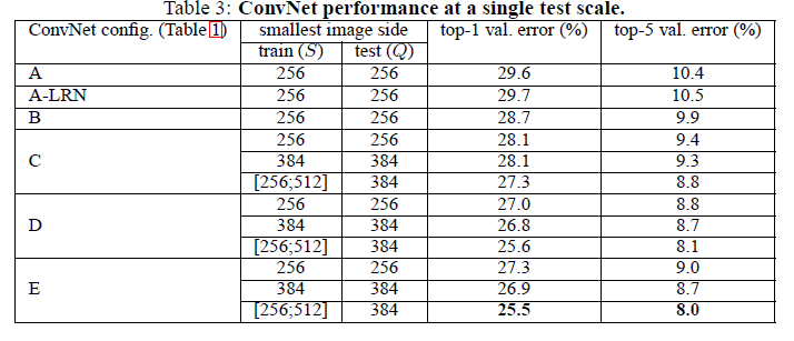
In the first part of the experiment, the test image size was set as Q = S for fixed S, and Q = 0.5(Smin + Smax) for jittered. One important result of this evaluation was that that the classification error decreases with the increased ConvNet depth. Moreover, The worse performance of the configuration with 1x1 filter (C ) in comparison with the one with 3x3 filter (D) indicates that while the additional non-linearity does help (C is better than B), it is also important to capture spatial context by using conv. filters with non-trivial receptive fields (D is better than C). Finally, scale jittering at training time leads to significantly better results than training on images with fixed smallest side. This confirms that training set augmentation by scale jittering is indeed helpful for capturing multi-scale image statistics.

Multi-Scale Evaluation

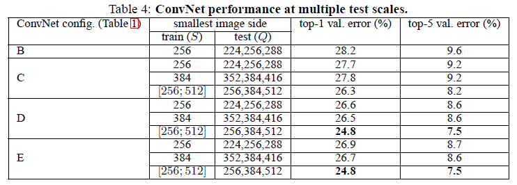
In addition to single scale evaluation stated in the previous section, in this paper, the effect of scale jittering at test time is assessed by running a model over several rescaled versions of a test image (corresponding to different values of Q), followed by averaging the resulting class posteriors. The results indicate that scale jittering at test time leads to better performance (as compared to evaluating the same model at a single scale).

Their best single-network performance on the validation set is 24.8%/7.5% top-1/top-5 error. On the test set, the configuration E achieves 7.3% top-5 error.

Comparison With The State Of The Art

Their very deep ConvNets significantly outperform the previous generation of models, which achieved the best results in the ILSVRC-2012 and ILSVRC-2013 competitions.

Appendix A: Localization

In addition to classification, the introduced architectures have been used for localization purposes. To perform object localisation, a very deep ConvNet, where the last fully connected layer predicts the bounding box location instead of the class scores is used. Apart from the last bounding box prediction layer, the ConvNet architecture D which was found to be the best-performing in the classification task is implemented and training of localisation ConvNets is similar to that of the classification ConvNets. The main difference is that the logistic regression objective is replaced with a Euclidean loss, which penalises the deviation of the predicted bounding box parameters from the ground-truth. Two testing protocols are considered: The first is used for comparing different network modifications on the validation set, and considers only the bounding box prediction for the ground truth class. (The bounding box is obtained by applying the network only to the central crop of the image.) The second, fully-fledged, testing procedure is based on the dense application of the localization ConvNet to the whole image, similarly to the classification task.

the localization experiments indicate that performance advancement brought by the introduced very deep ConvNets produces considerably better results with a simpler localization method, but a more powerful representation.

Conclusion

Very deep ConvNets are introduced in this paper. The results show that the configuration has good performance on classification and localization and significantly outperform the previous generation of models, which achieved the best results in the ILSVRC-2012 and ILSVRC-2013 competitions. Details and more results on these competitions can be found here.<ref> Russakovsky, Olga, et al. "Imagenet large scale visual recognition challenge." International Journal of Computer Vision (2014): 1-42. </ref> They also showed that their configuration is applicable to some other datasets.

Resources

The Oxford Visual Geometry Group (VGG) has released code for their 16-layer and 19-layer models. The code is available on their website in the format used by the Caffe toolbox and includes the weights of the pretrained networks.

References

<references />

Krizhevsky, A. One weird trick for parallelizing convolutional neural networks. CoRR, abs/1404.5997, 2014.