distributed Representations of Words and Phrases and their Compositionality
Introduction
This paper<ref> Mikolov, Tomas, et al. "Distributed representations of words and phrases and their compositionality." Advances in neural information processing systems. 2013. </ref> presents several extensions of the Skip-gram model introduced by Mikolov et al. <ref name=MiT> Mikolov, Tomas, et al "Efficient Estimation of Word Representations in Vector Space" in ICLR Workshop, (2013). </ref>. The Skip-gram model is an efficient method for learning high-quality vector representations of words from large amounts of unstructured text data. The word representations computed using this model are very interesting because the learned vectors explicitly encode many linguistic regularities and patterns. Somewhat surprisingly, many of these patterns can be represented as linear translations. For example, the result of a vector calculation vec(“Madrid”) - vec(“Spain”) + vec(“France”) is closer to vec(“Paris”) than to any other word vector. The authors of this paper show that subsampling of frequent words during training results in a significant speedup and improves accuracy of the representations of less frequent words. In addition, a simplified variant of Noise Contrastive Estimation (NCE) <ref name=GuM> Gutmann, Michael U, et al "Noise-contrastive estimation of unnormalized statistical models, with applications to natural image statistics" in The Journal ofMachine Learning Research, (2012). </ref>. for training the Skip-gram model is presented that results in faster training and better vector representations for frequent words, compared to more complex hierarchical softmax that was used in the prior work <ref name=MiT></ref>. It also shows that a non-obvious degree of language understanding can be obtained by using basic mathematical operations on the word vector representations. For example, vec(“Russia”) + vec(“river”) is close to vec(“Volga River”), and vec(“Germany”) + vec(“capital”) is close to vec(“Berlin”).
The Skip-gram Model
The training objective of the Skip-gram model is to find word representations that are useful for predicting the surrounding words in a sentence or a document. More formally, given a sequence of training words [math]\displaystyle{ w_1, w_2,..., w_T }[/math] the objective of the Skip-gram model is to maximize the average log probability:
[math]\displaystyle{
\frac{1}{T} \sum_{t=1}^{T} \sum_{-c\leq j\leq c} log(p(w_{t+j}|w_t))
}[/math]
where [math]\displaystyle{ c }[/math] is the size of the training context (which can be a function of the center word [math]\displaystyle{ w_t }[/math]) and [math]\displaystyle{ p(w_{t+j}|w_t) }[/math] is defined using softmax function:
[math]\displaystyle{ p(w_O|w_I) = \frac{exp ({v'_{W_O}}^T v_{W_I})}{\sum{w=1}^{W} exp ({v'_{W}}^T v_{W_I})} }[/math]
Here, [math]\displaystyle{ v_w }[/math] and [math]\displaystyle{ v'_w }[/math] are the “input” and “output” vector representations of [math]\displaystyle{ w }[/math], and [math]\displaystyle{ W }[/math] is the number of words in the vocabulary.
Hierarchical Softmax
Hierarchical Softmax is a computationally efficient approximation of the full softmax <ref name=MoF> Morin, Frederic, et al "Hierarchical probabilistic neural network language model" in Proceedings of the international workshop on artificial intelligence and statistics, (2015). </ref>. Hierarchical Softmax evaluate only about [math]\displaystyle{ log_2(W) }[/math] output nodes instead of evaluating [math]\displaystyle{ W }[/math] nodes in the neural network to obtain the probability distribution.
The hierarchical softmax uses a binary tree representation of the output layer with the [math]\displaystyle{ W }[/math] words as its leaves and, for each node, explicitly represents the relative probabilities of its child nodes. These define a random walk that assigns probabilities to words.
Let [math]\displaystyle{ n(w,j) }[/math] be the [math]\displaystyle{ j^{th} }[/math] node on the path from the root to [math]\displaystyle{ w }[/math], and let [math]\displaystyle{ L(w) }[/math] be the length of this path, so [math]\displaystyle{ n(w,1) = root }[/math] and [math]\displaystyle{ n(w,L(w)) = w }[/math]. In addition, for any inner node [math]\displaystyle{ n }[/math], let [math]\displaystyle{ ch(n) }[/math] be an arbitrary fixed child of [math]\displaystyle{ n }[/math] and let [math]\displaystyle{ [[x]] }[/math] be 1 if [math]\displaystyle{ x }[/math] is true and -1 otherwise. Then the hierarchical softmax defines [math]\displaystyle{ p(w_O|w_I ) }[/math] as follows:
[math]\displaystyle{ p(w|w_I) = \prod_{j=1}^{L(w)-1} \sigma ([[n(w,j+1)=ch(n(w,j))]]{v'_{n(w,j)}}^T v_{W_I}) }[/math]
where
[math]\displaystyle{ \sigma (x)=\frac{1}{1+exp(-x)} }[/math]
In this paper, a binary Huffman tree is used as the structure for the hierarchical softmax because it assigns short codes to the frequent words which results in fast training. It has been observed before that grouping words together by their frequency works well as a very simple speedup technique for the neural network based language models <ref name=MiT></ref><ref name=MiT2> Mikolov, Tomas, et al "Extensions of recurrent neural network language model." in Acoustics, Speech and Signal Processing (ICASSP), (2011). </ref>.
Negative Sampling
Noise Contrastive Estimation (NCE) is an alternative to the hierarchical softmax. NCE indicates that a good model should be able to differentiate data from noise by means of logistic regression. While NCE can be shown to approximately maximize the log probability of the softmax, the Skipgram model is only concerned with learning high-quality vector representations, so we are free to simplify NCE as long as the vector representations retain their quality. Negative sampling (NEG) is defined by the objective:
[math]\displaystyle{ log \sigma ({v'_{W_O}}^T v_{W_I})+\sum_{i=1}^{k} \mathbb{E}_{w_i\sim P_n(w)}[log \sigma ({-v'_{W_i}}^T v_{W_I})] }[/math]
The main difference between the Negative sampling and NCE is that NCE needs both samples and the numerical probabilities of the noise distribution, while Negative sampling uses only samples. And while NCE approximately maximizes the log probability of the softmax, this property is not important for our application.
Both NCE and NEG have the noise distribution [math]\displaystyle{ P_n(w) }[/math] as a free parameter. We investigated a number of choices for [math]\displaystyle{ P_n(w) }[/math] and found that the unigram distribution [math]\displaystyle{ U(w) }[/math] raised to the 3/4rd power (i.e., [math]\displaystyle{ U(w)^{3/4}/Z) }[/math] outperformed significantly the unigram and the uniform distributions, for both NCE and NEG on every task we tried including language modeling.
Subsampling of Frequent Words
In very large corpora, the most frequent words can easily occur hundreds of millions of times (e.g., “in”, “the”, and “a”). Such words usually provide less information about the surrounding words that rarer words (i.e., "the" provides little information about the next word because it co-occurs with a huge number of words), and the representation of the frequent word will be unlikely to change significantly after many iterations.
To counter the imbalance between the rare and frequent words, a simple subsampling approach is used. Each word [math]\displaystyle{ w_i }[/math] in the training set is discarded with probability computed by the formula:
[math]\displaystyle{ P(w_i)=1-\sqrt{\frac{t}{f(w_i)}} }[/math]
where [math]\displaystyle{ f(w_i) }[/math] is the frequency of word [math]\displaystyle{ w_i }[/math] and [math]\displaystyle{ t }[/math] is a chosen threshold, typically around [math]\displaystyle{ 10^{−5} }[/math].
Empirical Results
The Hierarchical Softmax (HS), Noise Contrastive Estimation, Negative Sampling, and subsampling of the training words are evaluated with the help of the analogical reasoning task1 <ref name=MiT></ref>. The task consists of analogies such as “Germany” : “Berlin” :: “France” : ?, which are solved by finding a vector x such that vec(x) is closest to vec(“Berlin”) - vec(“Germany”) + vec(“France”) according to the cosine distance. This specific example is considered to have been answered correctly if x is “Paris”. The task has two broad categories: the syntactic analogies (such as “quick” : “quickly” :: “slow” : “slowly”) and the semantic analogies, such as the country to capital city relationship.
For training the Skip-gram models, a large dataset consisting of various news articles is used (an internal Google dataset with one billion words). All words that occurred less than 5 times in the training data were discarded, which resulted in a vocabulary of size 692K. The performance of various Skip-gram models on the word analogy test set is reported in Table 1. The table shows that Negative Sampling outperforms the Hierarchical Softmax on the analogical reasoning task, and has even slightly better performance than the Noise Contrastive Estimation. The subsampling of the frequent words improves the training speed several times and makes the word representations significantly more accurate.

Learning Phrases
Many phrases have a meaning that is not a simple composition of the meanings of its individual words. To learn vector representation for phrases, we first find words that appear frequently together, and infrequently in other contexts. For example, “New York Times” and “Toronto Maple Leafs” are replaced by unique tokens in the training data, while a bigram “this is” will remain unchanged. This way, we can form many reasonable phrases without greatly increasing the size of the vocabulary; in theory, we can train the Skip-gram model using all n-grams, but that would be too memory intensive. A simple data-driven approach, where phrases are formed based on the unigram and bigram counts is applied to identify the phrases. In this approach, a score is calculated as:
[math]\displaystyle{ score(w_i,w_j)=\frac{count(w_iw_j)-\delta}{count(w_i)count(w_j)} }[/math]
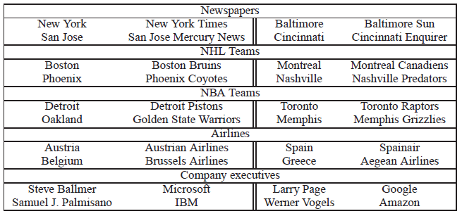
The [math]\displaystyle{ \delta }[/math] is used as a discounting coefficient and prevents too many phrases consisting of very infrequent words to be formed. The bigrams with scores above the chosen threshold are then used as phrases. The quality of the phrase representations is evaluated using a new analogical reasoning task that involves phrases. Table 2 shows examples of the five categories of analogies used in this task.

Phrase Skip-Gram Results
First, the phrase based training corpus is constructed and then Skip-gram models are trained using different hyperparameters. Table 3 shows the results using vector dimensionality 300 and context size 5. This setting already achieves good performance on the phrase dataset, and allowed us to quickly compare the Negative Sampling and the Hierarchical Softmax, both with and without subsampling of the frequent tokens. The results show that while Negative Sampling achieves a respectable accuracy even with k = 5, using k = 15 achieves considerably better performance. Also, the subsampling can result in faster training and can also improve accuracy, at least in some cases.

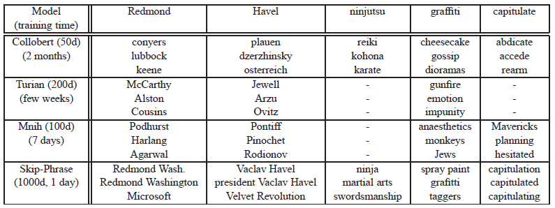
The amount of the training data was increased to 33 billion words in order to maximize the accuracy on the phrase analogy task. Hierarchical softmax, dimensionality of 1000, and the entire sentence for the context were used. This resulted in a model that reached an accuracy of 72%. Reducing the size of the training dataset to 6 billion caused lower accuracy (66%), which suggests that large amount of the training data is crucial. To gain further insight into how different the representations learned by different models are, nearest neighbors of infrequent phrases were inspected manually using various models. In Table 4 shows a sample of such comparison. Consistently with the previous results, it seems that the best representations of phrases are learned by a model with the hierarchical softmax and subsampling.

Additive Compositionality
The word and phrase representations learned by the Skip-gram model exhibit a linear structure that makes it possible to perform precise analogical reasoning using simple vector arithmetics. Also, the Skip-gram representations exhibit another kind of linear structure that makes it possible to meaningfully combine words by an element-wise addition of their vector representations. This phenomenon is illustrated in Table 5. The additive property of the vectors can be explained by inspecting the training objective. The word vectors are in a linear relationship with the inputs to the softmax nonlinearity. As the word vectors are trained to predict the surrounding words in the sentence, the vectors can be seen as representing the distribution of the context in which a word appears. These values are related logarithmically to the probabilities computed by the output layer, so the sum of two word vectors is related to the product of the two context distributions. The product works here as the AND function: words that are assigned high probabilities by both word vectors will have high probability, and the other words will have low probability.

Comparison to Published Word Representations
Table 6 shows the empirical comparison between different neural network-based representations of words by showing the nearest neighbors of infrequent words. These examples show that the big Skip-gram model trained on a large corpus visibly outperforms all the other models in the quality of the learned representations. This can be attributed in part to the fact that this model has been trained on about 30 billion words, which is about two to three orders of magnitude more data than the typical size used in the prior work. Interestingly, although the training set is much larger, the training time of the Skip-gram model is just a fraction of the time complexity required by the previous model architectures.

Conclusion
This work has the following key contributions:
1. This work shows how to train distributed representations of words and phrases with the Skip-gram model and demonstrate that these representations exhibit linear structure that makes precise analogical reasoning possible.
2. It is a computationally efficient model architecture which results in successfully train models on several orders of magnitude more data than the previously published models.
3. Introducing Negative sampling algorithm, which is an extremely simple training method that learns accurate representations especially for frequent words.
4. The choice of the training algorithm and the hyper-parameter selection is a task specific decision. It is shown that the most crucial decisions that affect the performance are the choice of the model architecture, the size of the vectors, the subsampling rate, and the size of the training window.
5. The word vectors can be meaningfully combined using just simple vector addition. Another approach for learning representations of phrases presented in this paper is to simply represent the phrases with a single token. Combining these two approaches gives a powerful yet simple way how to represent longer pieces of text, while having minimal computational complexity.
Le et al have used the idea of the current paper for learning paragraph vectors. In that later work they used paragraph vectors for prediction of the next word. Every word and also every paragraph is mapped to a unique vector in represented in a column of two different matrices W and D. Then paragraph vectors and word Le Q, Mikolov T. vectors are concatenated to contribute for predicting the next word [1]<ref> Distributed Representations of Sentences and Documents </ref>.
Recursive Autoencoder
This is taken from paper 'Semi-supervised recursive autoencoders for predicting sentiment distributions'.<ref> Socher, et al. [2] </ref>
Other techniques for sentence representation
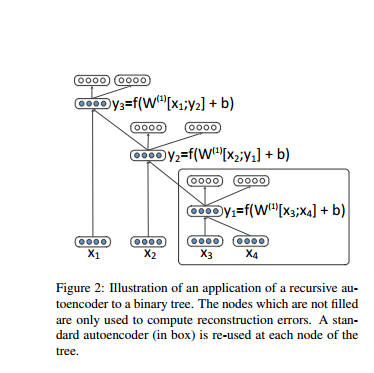
The idea of Recursive Autoencoder is summarized in the figure below. The example illustrates the recursive autoencoder to a binary tree.
Assume given a list of word vectors [math]\displaystyle{ x = (x_1, ..., x_m) }[/math], we need to branch triplets of parents with children: [math]\displaystyle{ (y_1 \rightarrow x_3x_4), (y_2 \rightarrow x_2y_1), (y_3 \rightarrow x_1y_2) }[/math].
The first parent [math]\displaystyle{ y_1 }[/math] is computed from the children [math]\displaystyle{ (c_1, c_2) = (x_3, x_4) }[/math]: [math]\displaystyle{ p=f(W^{(1)}[c_1; c_2] + b^{(1)}) }[/math] , where W is the parameter matrix and b is bias term.
The autoencoder comes in by reconstructing children set [math]\displaystyle{ [c_1^'; c_2^'] = W^{(2)}p + b^{(2)} }[/math]. The object of this method is to minimized the MSE of original children set and the reconstructed children set.
Resources
The code for training the word and phrase vectors based on this paper is available in the open source project word2vec. This project also contains a set of pre-trained 300-dimensional vectors for 3 million words and phrases.
References
<references />
