deep Learning of the tissue-regulated splicing code

Introduction

Alternative splicing(AS) is a regulated process during gene expression that enables the same gene to give rise to splicing isoforms containing different combinations of exons, which leads to different protein products. Furthermore, AS is often tissue dependent. This paper mainly focus on performing Deep Neural Network (DNN) in predicting outcome of splicing, and compare the performance to formerly trained model Bayesian Neural Network<ref>https://www.cs.cmu.edu/afs/cs/academic/class/15782-f06/slides/bayesian.pdf</ref> (BNN), and Multinomial Logistic Regression<ref>https://en.wikipedia.org/wiki/Multinomial_logistic_regression</ref> (MLR).

A huge difference that the author imposed in DNN is that each tissue type are treated as an input; while in previous BNN, each tissue type was considered as a different output of the neural network. Moreover, in previous work, the splicing code infers the direction of change of the percentage of transcripts with an exon spliced in (PSI). Now, this paper perform absolute PSI prediction for each tissue individually without averaging across tissues, and also predict the difference PSI ([math]\displaystyle{ \Delta }[/math]PSI) between pairs of tissues. Apart from regular deep neural network, this model will train these two prediction tasks simultaneously.

Model

The dataset consists of 11019 mouse alternative exons profiled from RNA-Seq<ref>https://en.wikipedia.org/wiki/RNA-Seq</ref> Data. Five tissue types are available, including brain, heart, kidney, liver and testis.

The DNN is fully connected, with multiple layers of non-linearity consisting of hidden units. The mathematical expression of model is below:

[math]\displaystyle{ {a_v}^l = f(\sum_{m}^{M^{l-1}}{\theta_{v,m}^{l}a_m^{l-1}}) }[/math]

where a is the weighted sum of outputs from the previous layer. [math]\displaystyle{ \theta_{v,m}^{l} }[/math] is the weights between layers.

[math]\displaystyle{ f_{RELU}(z)=max(0,z) }[/math]

The RELU unit was used for all hidden units except for the first hidden layer, which uses TANH units.

[math]\displaystyle{ h_k=\frac{exp(\sum_m{\theta_{k,m}^{last}a_m^{last}})}{\sum_{k'}{exp(\sum_{m}{\theta_{k',m}^{last}a_m^{last}})}} }[/math]

this is the softmax function of the last layer.

The cost function we want to minimize here during training is [math]\displaystyle{ E=-\sum_a\sum_{k=1}^{C}{y_{n,k}log(h{n,k})} }[/math], where [math]\displaystyle{ n }[/math] denotes the training example, and [math]\displaystyle{ k }[/math] indexes [math]\displaystyle{ C }[/math] classes.

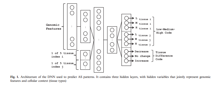
The identity of two tissues are then appended to the vector of outputs of the first hidden layer, together forming the input into the second hidden layer. The identity is a 1-of-5 binary variables in this case. (Demonstrated in Fig.1) The first targets for training contains three classes, which labeled as low, medium, high (LMH code). The second task describes the [math]\displaystyle{ \Delta PSI }[/math] between two tissues for a particular exon. The three classes corresponds to this task is decreased inclusion, no change and increased inclusion (DNI code).Both the LMH and DNI codes are trained jointly, reusing the same hidden representations learned by the model. The DNN used backpropagation with dropout to train the data, and used different learning rates for two tasks.

Training the model

The first hidden layer was trained as an autoencoder to reduce the dimensionality of the feature in an unsupervised manner. This method of pretraining the network has been used in deep architecture to initialize learning near a good local minimum. In the second stage of training, the weights from the input layer to the first hidden layer are fixed, and 10 additional inputs corresponding to tissues are appended. The vector representation for tissue is a binary vector. For example, it takes the form [0 1 0 0 0] to denote the second tissue out of five possible types. Moreover, the weights connected to the rest hidden layers of the DNN are then trained together in a supervised layers with backpropagation method. The DNN weights were initialized with small random values sampled from a zero-mean Gaussian distribution with 50% dropout rate for all layers except for the input layer.

In addition, they filtered the data first before training by excluding examples if the total number RNA-Seq junction reads is below 10. This removed 45.8% of the total number of training examples.

Both the LMH and DNI codes are trained together. Because each of these two tasks might be learning at different rates. This is to prevent one task from overfitting too soon and negatively affecting the performance of another task before the complete model is fully trained.

The targets consist of (i) PSI for each of the two tissues and (ii) [math]\displaystyle{ \deltaPSI }[/math] between the two tissues. As a result, given same tissues, the model should predict no change for [math]\displaystyle{ \deltaPSI }[/math]. Also, if the tissues are swapped in the input, the previous increased inclusion label should become decrease.

Performance comparison

The performance of the model was assessed using the area under the Receiver-Operating Characteristic curve (AUC) metric. This paper compared three methods through the same baseline, DNN, BNN and MLR.

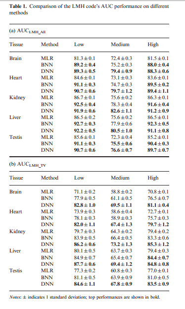
The result (LMH code) shows in the table below. Table 1a reports AUC for PSI predictions from the LMH code on all tissues; while 1b reports AUC evaluated on the subset of events that exhibit large tissue variability. From 1a, the performance of DNN in low and high categories are comparable with the BNN, but outperformed at the medium level. From 1b, DNN significantly outperformed BNN and MLR. In both comparison, MLR performed poorly.

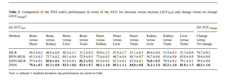
Next, we look at how well the different methods can predict [math]\displaystyle{ \Delta PSI }[/math] (DNI code). DNN predicts LMH code and DNI code at the same time; while in BNN, the model can only predict LMH code. Thus, for a fair comparison. author used a MLR on the predicted outputs for each tissue pair from BNN and similarly trained MLR on the LMH outputs of the DNN. Table 2 shows that both DNN and DNN+MLR outperformed the BNN+MLR or MLR.

Why did DNN outperform?

1. The use of tissue types as an input freature, which stringently required the model's hidden representations be in a form that can be well-modulated by information specifying the different tissue types for splicing pattern prediction.

2. The model is described by thousands of hidden units and multiple layers of non-linearity. In contrast, BNN only has 30 hidden units, which may not be sufficient.

3. A hyperparameter search is performed to optimize the DNN.

4. The use of dropout, which contributed ~1-6% improvement in the LMH code for different tissues, and ~2-7% in the DNI code, compared with without dropout.

5. Training was biased toward the tissue-specific events (by construction of minibatches).

Conclusion

This work shows that DNN can also be used in a sparse biological dataset. Furthermore, the input features can be analyzed in terms of the predictions of the model to gain some insights into the inferred tissue-regulated splicing code. This architecture can easily be extended to the case of more data from different sources.

reference

<references />