the Wake-Sleep Algorithm for Unsupervised Neural Networks

Introduction

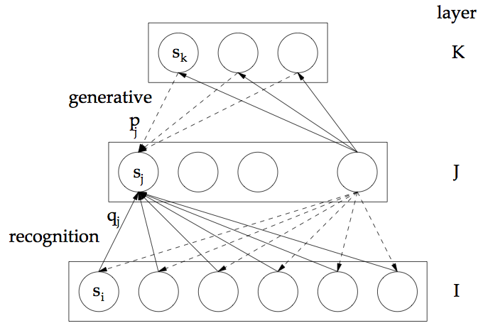
In considering general learning procedures, supervised methods for neural networks are limited in that they can only be executed in specifically-structured environments. For these systems to learn, the environment must be equipped with an external "teacher" providing the network with explicit feedback on its predictive performance. From there, the system needs a means for circulating this error information across the entire network, so that the weights can be adjusted accordingly. To apply neural networks in contexts not satisfying these specific requirements, the authors purpose the wake-sleep algorithm, a two-phase procedure in which each network layer effectively learns representations of the activity in adjacent hidden layers. Here, the network is composed of feed-forward "recognition" connections used to generate an internal representation of the input, and feed-back generative connections used to produce an estimated reconstruction of the original input based on this learned internal representation. The goal is to learn an efficient representation which accurately characterizes the input to the system.

Model Structure

The wake-sleep algorithm is used to train Helmholtz machines, networks possessing the feed-forward and feed-back connections as described above. In deploying a Helmholtz machine, we hope to encode an abstraction capturing the relevant properties of the data, and using this representation, find a generative reconstruction of the original input. This is analogous to learning a data-driven "bottom-up" representation of the input that is used to inform the higher-order "top-down" reconstruction.

Figure 1: The Helmholtz network structure.

Selecting a Cost

To enforce the requirement that the network produces efficient reconstructions of the data, the cost function is selected by viewing the problem as a task of information transmission. In this task, the original input vector is to be indirectly communicated from the sender to the receiver via first sending the internal representation of the datum learned by the system, and then passing along the deviation of the original input from its approximation produced by the generative reconstruction of the internal representation. Naturally, the objective then becomes to minimize the length of the sequence of bits that is needed to express the original input in this indirect manner. This corresponds to adopting the minimum description length (MDL) principle to guide the process of learning the representation. MDL is a general methodological principle stating that among a set of candidate models for the data, the one which can be represented in the fewest number of bits in the process of communication ought to be selected (see http://papers.nips.cc/paper/798-autoencoders-minimum-description-length-and-helmholtz-free-energy.pdf).

In order to see how the MDL criterion is to be implemented in this context, we must first specify a more precise network structure and the procedure which generates the reconstruction. The authors restrict the network to consist of stochastic binary units taking values in {0,1}, where the probability of unit v being active is given by

[math]\displaystyle{ P(s_v = 1) = (1 + exp(-b_v - \sum_{u}^{} s_u w_{uv}))^{-1} }[/math] (1)

Here, [math]\displaystyle{ b_v }[/math] is the additive constant for unit v, and [math]\displaystyle{ w_{uv} }[/math] is the weight associated with the connection to unit u. For the bottom-up recognition connections, the units u which are summed over are from the immediately-preceding hidden layer, whereas these units will be from the immediately-following layer for the top-down generative connections.

Now, to produce a reconstruction of a particular input, we first feed the input into the network, using the recognition weights to activate the units of each successive layer until the highest hidden layer is reached. With multiple hidden layers, this process is analogous to creating a hierarchy of representations; the first hidden layer generates a representation of the original input, the second layer produces a representation of the representation provided to it by the first layer, and each additional layer similarly provides a higher-order meta-representation of the input. At the final layer, the network begins the process of using this set of representations to express the approximation via the generative connections. To do this, for each unit of the top layer, the sigmoid function is simply applied to the additive constant in (1), as there are no subsequent layers providing influence. Then, for each lower layer, the activation probabilities of its units are computed using (1), where the u 's are the set of units in the next-highest layer.

The collection of states [math]\displaystyle{ s_j }[/math] of the binary units with corresponding activation probabilities [math]\displaystyle{ p_j }[/math] for the representation produced by this process now gives us a means to quantify the description length of the representation. We know that in order to represent the state of the stochastic binary unit j, we require [math]\displaystyle{ C(s_j) := -s_jlog p_j - (1 - s_j)log (1 - p_j) }[/math] bits. So, for an input d, the total description length for representing d in terms of its learned representation [math]\displaystyle{ \alpha }[/math] is the sum of the description lengths for the individual hidden units of the network plus the description length of the procedure for decoding the original input given the hidden representation:

[math]\displaystyle{ C(\alpha , d) = \sum_{j}^{}C(s_j^{\alpha}) + \sum_{i}^{}C(s_i^d | d) }[/math]

Recalling that the hidden units are stochastic, it is clear that a given input vector will have a broad array of possible network representations, making the recognition weights specify a distribution [math]\displaystyle{ Q(\alpha | d) }[/math] over representations of the input. Taking this into account, we realize that the cost function for representing an input d will be a representation cost averaged over the possible representations of d. If we also consider the entropy associated with the variability in representing d, the overall cost for representing d becomes [math]\displaystyle{ C(d) = \sum_{\alpha}^{} Q(\alpha | d)C(\alpha , d) - (- \sum_{\alpha}^{} Q(\alpha | d)log Q(\alpha | d)) }[/math]; namely, the expected description length for representing d subtracted by the entropy in representation.

Minimizing the Cost

It turns out that the representation cost we specified is related to the notion of Helmholtz free energy in statistical physics. Analogous to this context, we find that the cost is minimized by setting the probability of a representation to be proportionate to an exponential function of its cost:

[math]\displaystyle{ P(\alpha | d) = \frac {exp(-C(\alpha, d))}{\sum_{\beta}^{} exp(-C(\beta, d))} }[/math]

This corresponds to the Boltzmann distribution with temperature parameter set to 1. Essentially, this means that rather than attempting to minimize the description cost of any single particular representation of an input, we should seek to find recognition weights which allows [math]\displaystyle{ Q( \alpha |d) }[/math] to be a good approximation of this Boltzmann distribution. Given this cost and general criterion for minimizing it, we can now turn to the two-phase procedure used to determine the network weights.

The Wake Phase

As suggested by the name, in this stage, the network is receptive to external input. The system will receive input vectors which will be converted into internal representations across the hidden layers. To allow the input to propagate forwards through the network, the bottom-up recognition weights must be held fixed. Consequently, after an input vector has been processed in a bottom-up manner, we naturally seek to minimize top-down reconstruction error, the error incurred in using a layer's learned representation to predict the configuration in the layer below it. This is accomplished by updating the generative weights using the derivative of the description cost [math]\displaystyle{ C( \alpha , d) }[/math] with respect to the generative weights, for the learned representation [math]\displaystyle{ \alpha }[/math]. Using the purely local delta rule, this term for the top-down weight on the connection from k to j becomes:

[math]\displaystyle{ \Delta w_{kj} = \epsilon s_k^{\alpha}(s_j^{\alpha} - p_j^{\alpha}) }[/math].

We see that this term encourages each hidden layer to improve its performance in predicting the states of the layer immediately beneath it.

The Sleep Phase

While the wake phase involved processing external input for the purpose of improving the top-down reconstructions of it, the sleep phase closes the network off to external input and seeks to improve the performance of the recognition weights using only the current internal generative model of the world that has been learned. We recall that adjustment of the recognition weights is a necessary step, as the wake phase only considers the particular learned representation of the data d, whereas we seek to minimize the total cost [math]\displaystyle{ C(d) }[/math] across all possible representations of d. It is this step which encourages the distribution over representations [math]\displaystyle{ Q(\alpha | d) }[/math] to greater resemble the Boltzmann distribution. The idea is that, given we have tuned a generative model of the input in the wake phase, we can simulate external input to the network by sampling from these generative models, and see how the recognition weights perform in representing these simulated cases. Beginning at the highest layer, we use its stochastic units to generate a "fantasy" input, propagating this fantasy back down through the network using the generative connections. From there, we update the bottom-up weights with the objective of maximizing the log probability of capturing the states of the hidden units which generated this fantasy input. This involves computing the weight-adjustment term [math]\displaystyle{ \Delta w_{jk} = \epsilon s_j^{\gamma} (s_k^{\gamma} - q_k^{\gamma}) }[/math], where [math]\displaystyle{ \gamma }[/math] determines the states of the hidden and input units for a given fantasy, and [math]\displaystyle{ q_k^{\gamma} }[/math] is the probability of unit k being activated as a result of applying the recognition weights to generate a state [math]\displaystyle{ s_j^{\gamma} }[/math] of node j in the layer below.

We can see that the sleep phase tunes the recognition weights by considering their performance on hypothetical input drawn from the network's generative model of the input. This is a proxy for the objective of obtaining recognition weights that are well-calibrated to the true external input being considered. An obvious limitation in this approximation is that, in the early stages of training, the network's generative model will likely be a poor representation of the true distribution of the input, meaning that the recognition weights will be adjusted based on data which is largely uncharacteristic of the training set.

Model Limitations

Due to the network structure, the distribution over representations [math]\displaystyle{ Q(\alpha | d) }[/math] is constrained to be a factorial distribution, as the states of units within the same hidden layer are independent when conditioned on the nodes of the layer below. This distributional form is advantageous in the sense that for a layer consisting of n hidden units, the probability distribution for the [math]\displaystyle{ 2^n }[/math] hidden states can be determined by providing n values, as opposed to [math]\displaystyle{ 2^n - 1 }[/math]. On the other hand, this conditional independence property also prohibits the model from representing "explaining-away" effects, a type of relation in which the states of one layer can be efficiently represented by only activating exactly one of two units in the following layer. However, the authors argue that the limitation of [math]\displaystyle{ Q(\alpha | d) }[/math] to be a factorial distribution is not completely debilitating, as, in the wake phase, the generative weights are adjusted to make the generative model similar to [math]\displaystyle{ Q(\alpha | d) }[/math]. In this sense, the generative model is encouraged to approximate the factorial form [math]\displaystyle{ Q(\alpha | d) }[/math], which limits issues surrounding the discrepancies between these distributions.

Empirical Performance

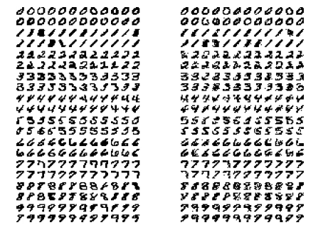
To examine the strength of the approximations adopted in their approach, the wake-sleep procedure was implemented in a task of hand-written digit-recognition. In addition to achieving accurate compressions of the data, Figure 2 below displays the interesting result illustrating that, after the completion of learning, the internal generative model has been tuned to produce accurate fantasy digits.

Figure 2: Input digits (left) as compared to simulated fantasy digits (right).

References

1. Hinton GE, Dayan P, Frey BJ, Neal RM. The Wake-Sleep Algorithm for Unsupervised Neural Networks. Science 26, May 1995. DOI: 10.1126/science.7761831

2. Hinton GE, Zemel RS. Autoencoders, Minimum Description Length, and Helmholtz Free Energy. Advances in Neural Information Processing Systems 6 (NIPS 1993).