strategies for Training Large Scale Neural Network Language Models
Introduction
Statistical models of natural languages are a key part of many systems today. The most widely used known applications are automatic speech recognition, machine translation, and optical character recognition. In recent years language models, including Recurrent Neural Network and Maximum Entropy-based models have gained a lot of attention and are considered the most successful models. However, the main drawback of these models is their huge computation complexity.
Motivation
As computational complexity is an issue for different types of deep neural network language models, this study briefly presents simple techniques that can be used to reduce computational cost of the training and test phases. The study also mentions that training neural network language models with maximum entropy models leads to better performance in terms of computational complexity.
Model description
Recurrent Neural Network Models
Features in this model are learned as a function of history. The model is described as:
[math]\displaystyle{ P(w|h)=\frac{e\sum_{k=1}^N \lambda_i f_i(s,w)} {\sum_{w=1} e \sum_{k=1}^N\lambda_i f_i(s,w)} }[/math]
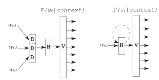
where f is a set of feature, λ is a set of weights, and s is a state of the hidden layer. The state of hidden layer can depend on the most recent word and the state in the previous time step. This recurrence allows the hidden layer to represent low-dimensional representation of the entire history.

Feedforward neural network 4-gram model (on the left) and Recurrent neural network language model (on the right)
Maximum Entropy model
A maximum entropy model has the following form:
[math]\displaystyle{ P(w|h)=\frac{e\sum_{k=1}^N \lambda_i f_i(h,w)} {\sum_{w=1} e \sum_{k=1}^N\lambda_i f_i(h,w)} }[/math]
where h is a history. Training maximum entropy model consists of learning the set of weights λ.
Computational complexity
The training time of N-gram neural network language model is proportional to:
[math]\displaystyle{ I*W*((N-1) *D*H+H*V) }[/math]
where I is the number of training epochs before convergence is achieved, W is the number of tokens in the training set, N is the N-gram order, D is the dimensionality of words in the low-dimensional space, H is size of the hidden layer and V size of the vocabulary.
The recurrent NN LM has computational complexity as:
[math]\displaystyle{ I*W*(H*H+H*V) }[/math]
It can be seen that by increasing order N, the complexity of the feedforward architecture increases linearly, while it remains constant for the recurrent one.
The computational complexity in maximum entropy model is also described as follows:
[math]\displaystyle{ I*W*(N*V) }[/math]
The simple techniques used in the present study to reduce the computational complexity are:
A. Reduction of training epochs
In this study, it is been demonstrated that good performance can be achieved while performing as few as 7 training epochs instead of using thousands of epochs.
B. Reduction of number of training tokens
In this study, NN LMs are trained only on small part of data (which are in-domain corpora) plus some randomly subsampled part of out-of-domain data.
C. Reduction of vocabulary
Goodman’s trick can be used for speeding up the models in terms of vocabulary. Each word from the vocabulary is assigned to a class and only the probability distribution over classes is computed.
Another way to reduce H×V is to choose a small value of H.
E. Parallelization
As the state of the hidden layer depends on the previous state, the recurrent networks are hard to be parallelized. One can parallelize just the computation between hidden and output layers.
Automatic data selection and sorting
The full training set is divided into 560 equally-sized chunks, and the perplexity on the development data is computed on each chunk. The data chunks with perplexity above 600 are discarded to obtain the reduced sorted training set.
Experiment with large RNN models
By training RNN model on the reduced sorted dataset and increasing the hidden layer, better results than baseline backoff model are obtained. However, the performance of RNN models is strongly correlated with the size of the hidden layer. Combining the RNN models with baseline 4-gram model and tuning the weights of individual models on the development set leads to quite impressive reduction of WER.
Hash-based implementation of class-based maximum entropy model
The maximum entropy model can be seen in the context of neural network models as a weight matrix that directly connects the input and output layers. In the present study, direct connections are added to the class-based RNN architecture. Direct parameters are used to connect input and output layers, and input and class layers. This model is denoted as RNNME.
Using direct connections leads to problems in memory complexity. To avoid this problem, a hash function is used to map the huge sparse matrix into one dimensional array. Using the underlying method, the achieved perplexity is better than the baseline perplexity of the KN4 model. Even better results are gained after interpolation of both models, and using rescoring experiment.
References
T. Mikolov, S. Kombrink, L. Burget, J. Cernocky ́, and S. Khudanpur, “Extensions of recurrent neural network language model,” in Proceed- ings of ICASSP, 2011.
T. Mikolov, M. Karafia ́t, L. Burget, J. Cˇernocky ́, and S. Khudanpur, “Recurrent neural network based language model