human-level control through deep reinforcement learning

Introduction

Reinforcement learning is "the study of how animals and artificial systems can learn to optimize their behaviour in the face of rewards and punishments" <ref>Dayan, Peter and Watkins, Christopher. "Reinforcement Learning." Encyclopedia of Cognitive Science.</ref>. Attempting to teach a dog a new trick is an example of this type of learning in animals, as the dog will (hopefully) learn that when it does the desired trick, it obtains a reward. The process is similar in artificial systems. For a given task, the algorithm for reinforcement learning selects an action that maximizes the expected cumulative future reward at every step in time, given the current state of the process. Then, it will carry out this action, observe the reward, and update the model to incorporate information about the reward generated by the action. The natural connection to neuroscience and animal behaviour makes reinforcement learning an attractive machine learning paradigm.

When creating artificial systems based on machine learning, however, we run into the problem of finding efficient representations from high-dimensional inputs. Furthermore, these representations need to use high-dimensional information from past experiences and generalize to new situations. The human brain is adept at this type of learning, using systems involving dopamine in the neurons with a similar structure to reinforcement learning algorithms <ref> Schultz, W., Dayan, P. & Montague, P. R. A neural substrate of prediction and reward. Science 275, 1593–1599 (1997) </ref>. Unfortunately, previous models have only been able replicate the success of humans on fully-observable, low-dimensional problems, such as backgammon <ref> Tesauro, Gerald. TD-Gammon, a self-teaching backgammon program, achieves master's play. AAAI Techinical Report (1993)</ref>.

In the paper that is summarized below <ref name = "main">Mnih, Volodymyr et. al. "Human-level control through deep reinforcement learning." Nature 518, 529-533 (2015) </ref>, a new structure called a deep Q-network (DQN) is proposed to handle high-dimensional inputs directly. The task that the DQN model is tested on is playing Atari 2600 games, where the only input data are the pixels displayed on the screen and the score of the game. It turns out that the DQN produces state-of-the-art results in this particular task, as we will see.

Problem Description

The goal of this research is to create a framework that would be able to excel at a variety of challenging learning tasks - a common goal in artificial intelligence. To that end, the DQN network is proposed, which combines reinforcement learning with deep neural networks <ref name = "main"></ref>. In particular, a deep convolutional network will be used to approximate the so-called optimal action-value function

[math]\displaystyle{ Q^*\left(s,a\right) = \max_\pi \mathop{\mathbb{E}}\left[r_t + \gamma r_{t+1} + \gamma^2 r_{t+2} + \ldots | s_t=s, a_t=a, \pi\right] }[/math]

which is the maximum cumulative sum of rewards [math]\displaystyle{ r_t\, }[/math] discounted by [math]\displaystyle{ \,\gamma }[/math] at each timestep [math]\displaystyle{ t\, }[/math]. This sum can be achieved from a policy [math]\displaystyle{ \pi = P\left(a|s\right) }[/math] after making an observation [math]\displaystyle{ \,s }[/math] and taking an action [math]\displaystyle{ \,a }[/math] <ref name = "main"></ref>.

Instability of Neural Networks as Function Estimate

Unfortunately, current methods which use deep networks to estimate [math]\displaystyle{ Q\, }[/math]suffer from instability or divergence for the following reasons:

1. Correlation within sequence of observations
2. Small updates to [math]\displaystyle{ Q\, }[/math]can significantly change the policy, and thus the data distribution
3. The action values [math]\displaystyle{ Q\, }[/math]are correlated with the target values [math]\displaystyle{ \,y = r_t + \gamma \max_{a'}Q(s', a') }[/math]

Overcoming Instability

One method of overcoming this instability is through the use of a biologically-inspired mechanism called experience replay. This involves storing [math]\displaystyle{ e_t = \left(s_t, a_t, r_t, s_{t+1}\right) }[/math] - known as the "experiences" - at each time step in a dataset [math]\displaystyle{ D_t = \left(e_1, e_2, \ldots, e_t\right) }[/math]. Then, during each learning update, minibatch updates are performed, where points are sampled uniformly from [math]\displaystyle{ \,D_t }[/math]. In practice, only [math]\displaystyle{ N }[/math] experiences are stored, where [math]\displaystyle{ N }[/math] is some large, finite number (e.g. [math]\displaystyle{ N=10^6 }[/math]). Incorporating experience replay into the algorithm removes the correlation between observations and smooths out the data distribution, since it takes an average over the past [math]\displaystyle{ N }[/math] states. This makes it much more unlikely that instability or divergence will occur.

This approach has several advantages over standard online Q-learning. First, each step of experience is potentially used in many weight updates, which allows for greater data efficiency. Second, learning directly from consecutive samples is inefficient, owing to the strong correlations between the samples; randomizing the samples breaks these correlations and therefore reduces the variance of the updates. Third, when learning on-policy the current parameters determine the next data sample that the parameters are trained on.

Another method used to combat instability is to use a separate network for generating the targets [math]\displaystyle{ y_i }[/math] as opposed to the same network. This is implemented by cloning the network [math]\displaystyle{ \,Q }[/math] every [math]\displaystyle{ \,C }[/math] iterations, and using this static, cloned network to generate the next [math]\displaystyle{ \,C }[/math] target values. Thus, the target network parameters are only updated with the Q-network parameters every [math]\displaystyle{ \,C }[/math] steps and are held fixed between individual updates. This additional modification reduces correlation between the target values and the action values, providing more stability to the network. In this paper, [math]\displaystyle{ \,C = 10^4 }[/math].

They also found that clipping the error term to be between -1 and 1 can further improve the stability of the algorithm.

Data & Preprocessing

The data used for this experiment is initially frame-by-frame pixel data from the Atari 2600 emulator, along with the game score (and the number of lives in applicable games). The frames are 210 x 160 images with colour, so some preprocessing is performed to simplify the data. The first step to encode a single frame is to take the maximum value for each pixel colour value over the frame being encoded and the previous frame <ref name = "main"></ref>. This removes flickering between frames, as sometimes images are only shown on every even or odd frame. Then, the image is converted to greyscale and downsampled to 84 x 84. This process is applied to the [math]\displaystyle{ m }[/math] most recent frames (here [math]\displaystyle{ m=4 }[/math]), and these 84 x 84 x 4 images are the inputs to the network.

Model Architecture

The framework for building an agent that can learn from environmental inputs is an iterative reward-based system. The agent will perform actions and constantly re-assess how its actions have affected its environment. To model this type of behaviour, the agent attempts to build up a model that relates actions to rewards over time. The underlying model relating actions to rewards, [math]\displaystyle{ Q }[/math], is estimated by a deep convolutional network, and is updated at every step in time.

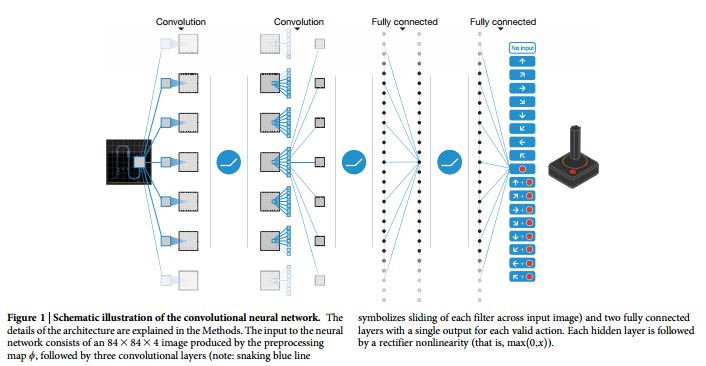
The structure of the network itself is as follows. There are separate output units for each possible action, and the only input to the network is the state representation. The outputs are the predicted Q-values for each action performed on the input state. The first hidden layer convolves 32 8x8 filters with stride 4, then applies a rectified nonlinear function <ref>Jarrett K. et. al. What is the best multi-stage architecture for object recognition? Proc. IEEE Int. Conf. Comput. Vis. 2146-2153 (2009)</ref>. In the next hidden layer, 64 4x4 filters with stride 2 are convolved and again followed by rectified non-linearity. The next layer is the final convolutional layer, with 64 3x3 filters of stride 1, followed by the rectifier. The final hidden layer in the network is fully-connected, with 512 rectifying units. The output layer is a fully-connected linear layer with a single output for each valid action, of which there ranged from 4 to 18 in any particular game<ref name = "main"></ref>.

Training

Framework and Additional Setup Details

Forty-nine Atari games were considered as experiments. A unique DQN is trained for each game, but the same structure, algorithm, and global parameters (e.g. [math]\displaystyle{ C }[/math] or [math]\displaystyle{ m }[/math] as above, among others) were used throughout. The value of the global parameters was selected by performing an informal search on a small subset of the 49 games. The goal is to use minimal prior knowledge and perform end-to-end training of these models based on game experience.

The reward structure for games was slightly changed, clipping negative rewards at -1 and positive rewards at 1, since score varies from game to game. This could be problematic since the agent may not properly prioritize higher-scoring actions, but it also helps stabilize the network and allows it to generalize to more games. However, the game itself is not otherwise changed.

There is also a frame-skipping technique employed, in which the agent only performs an action every [math]\displaystyle{ k^{th} }[/math] frame to allow the agent to play [math]\displaystyle{ k }[/math] times more games, as the network does not have to be trained on the skipped frames ([math]\displaystyle{ k=4 }[/math] here). Furthermore, I believe this creates a more realistic experience for the agent, as human players would not be able to change their own actions every single frame.

The agents are trained on 50 million frames of game play, which is about 38 days. The RMSProp <ref>Hinton, Geoffrey et al.Overview of Minibatch Gradient Descent. University of Toronto.</ref> algorithm, which performs stochastic gradient descent in small batches, is used to train the network.

Algorithm Background

Markovian Decision Process

A Markovian Decision Process is described by:

• A set of states [math]\displaystyle{ S }[/math]
• A set of actions [math]\displaystyle{ A }[/math]
• Stochastic transition [math]\displaystyle{ p(s, a, s') }[/math], describing the stochastic system
• Cost function [math]\displaystyle{ c: S X A \mapsto R }[/math]
• Policy [math]\displaystyle{ \pi^{*}: S \mapsto A }[/math]

The objective is to find the optimal policy [math]\displaystyle{ \pi }[/math] that minimizes the cost function [math]\displaystyle{ c }[/math].

Q Learning

Q learning is a reinforcement learning that is used to find an optimal policy (sequence of actions) for any Markov Decisoin Process (MDP). The Q learning algorithm at its core computes the best sequence of future actions based on previous states. It is an incremental Dynamic Programming procedure where all possible states has to be computed and stored in a table to find an optimal policy.

[math]\displaystyle{ Q_{k+1}(s, a) := (1 - \alpha) Q(s, a) + \alpha(c(s, a) + \gamma \min_{b} Q_{k}(S^{'}, b)) }[/math]

Where:

• [math]\displaystyle{ s }[/math]: state where the transition starts
• [math]\displaystyle{ a }[/math]: action applied
• [math]\displaystyle{ s' }[/math]: resulting state
• [math]\displaystyle{ \alpha }[/math]: learning parameter
• [math]\displaystyle{ \gamma }[/math]: discount factor (between 0 (short-term) and 1 (long-term))

Typically Q-learning is performed on-line. Riedmiller (2005) <ref>Riedmiller, Martin. "Neural fitted Q iteration–first experiences with a data efficient neural reinforcement learning method." Machine Learning: ECML 2005. Springer Berlin Heidelberg, 2005. 317-328.</ref> argues that in principle while Q-learning can be directly implemented in a neural network, the problem with online approach is it creates unstable results. Intuitively this makes sense because if Q-learning were to be used for controls, 1 sample point is not indicative whether the action applied is optimal or not. For reasons listed above Mnih et al (2015) <ref>Mnih, Volodymyr, et al. "Human-level control through deep reinforcement learning." Nature 518.7540 (2015): 529-533.</ref> devised a Q-learning updates on minibatches of experience.

Q-Iteration Learning

At each step in time, the agent selects an action [math]\displaystyle{ a_t\, }[/math] from the set of legal game actions [math]\displaystyle{ \mathbb{A} }[/math]. The agent observes an image [math]\displaystyle{ x_t \in \mathbb{R}^d }[/math] from the emulator, along with a reward [math]\displaystyle{ r_t\, }[/math]. It is impossible to fully understand the current game situation from a single screen, so a sequence of actions and observations [math]\displaystyle{ s_t = x_1, a_1, x_2, \ldots, a_{t-1}, x_t }[/math] is the input state.

Recall that if we define [math]\displaystyle{ R_t = \sum_{t'=t}^T \gamma^{t'-t}r_t }[/math], where [math]\displaystyle{ \gamma\, }[/math] is the discount factor and [math]\displaystyle{ \,T }[/math] is the step in which the game terminates, then

[math]\displaystyle{ Q^*\left(s,a\right) = \max_\pi \mathop{\mathbb{E}}\left[R_t| s_t=s, a_t=a, \pi\right] }[/math]

is the optimal action-value function.

The Bellman Equation in the Loss Framework

The optimal action-value function obeys the Bellman Equation:

[math]\displaystyle{ Q^*\left(s,a\right) = \mathop{\mathbb{E}_{s'}}\left[r + \gamma \max_{a'}Q^*\left(s',a'\right) | s, a\right] }[/math]

The intuition behind this identity is as follows: if the optimal value [math]\displaystyle{ Q^*(s',a')\, }[/math] at the next time step was known for all possible actions [math]\displaystyle{ a' }[/math], then the optimal strategy is to select the action [math]\displaystyle{ a' }[/math] maximizing the expected value above <ref name = "main"> </ref>. Using the Bellman Equation as an iterative update formula is impractical, however, since the action-value function is estimated separately for each sequence and cannot generalize.

It is necessary, in practice, to operate with an approximation of the action-value function. When a neural network with weights [math]\displaystyle{ \,\theta }[/math] is used, it is referred to as a Q-Network. A Q-Network is trained by adjusting [math]\displaystyle{ \,\theta_t }[/math] to reduce the mean-squared error in the Bellman Equation. The new target values for training are given by [math]\displaystyle{ y = r + \gamma\max_{a'} Q\left(s', a'; \theta_t^-\right) }[/math], where [math]\displaystyle{ \theta_t^-\, }[/math] are the parameters from some previous iteration.

The Full Algorithm

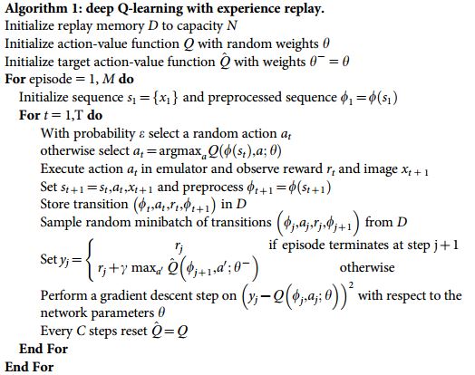
Now, with all the background behind us, the full Deep Q-Learning with Experience Replay algorithm is presented below:

Some notes about the algorithm:

• Replay memory is used to implement the experience replay technique described above
• An episode is one game
• Correlations between target values and the action function [math]\displaystyle{ Q\, }[/math]are mitigated by using [math]\displaystyle{ \hat{Q} }[/math] for the target values
  • Only updated every [math]\displaystyle{ \,C }[/math] steps

Results

Evaluation Procedure

The trained networks played each game 30 times, up to 5 minutes at a time. The random agent, which is the baseline comparison, chooses a random action every 6 frames (10 Hz). The human player uses the same emulator as the agents, and played under controlled conditions (most notably without sound). The human performance is the average reward from around 20 episodes of the game lasting up to 5 minutes, after 2 hours of practice playing each game. The human performance is set to be 100%, and the random agent has performance set to 0%.

Raw Score Results

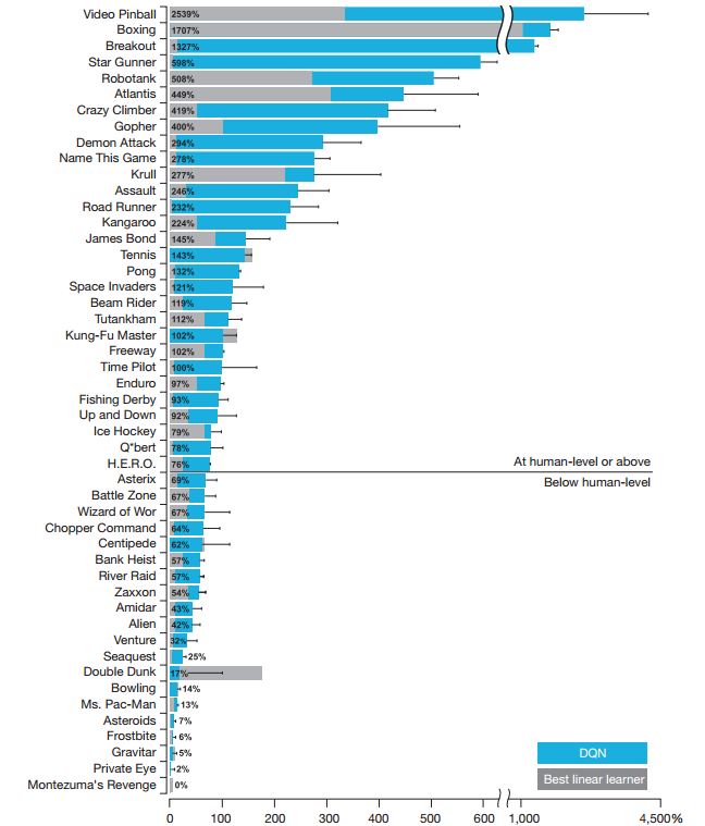
The DQN agent outperforms the best existing reinforcement learning methods on 43 of the games without incorporating prior knowledge about Atari games. Furthermore, the agent scores at least 75% of the human score on more than half of the games. Also, DQN performs well across a number of types of games. However, games which involve extended planning strategies still pose a major problem to DQN (e.g. Montezuma's Revenge). These results are visualized in the figure below:

Results with model components removed

Two important advances in this paper were presented: experience replay and creating a separate network to evaluate the targets. To visualize the impact of these advances, the network was trained with and without both of these concepts, and evaluated on its performance in each case. The results are shown in the table below, in percentage form as above:

Game	With Replay and Target Q	With Replay, Without Target Q	Without Replay, With Target Q	Without Replay, Without Target Q
Breakout	316.8	240.7	10.2	3.2
Enduro	1006.3	831.4	141.9	29.1
River Raid	7446.6	4102.8	2867.7	1453.0
Seaquest	2894.4	822.6	1003.0	275.8
Space Invaders	1088.9	826.3	373.2	302.0

Clearly, experience replay and maintaining a secondary network for computing target values are important. From these results, it seems that experience replay is more important on its own, except in Seaquest.

Conclusion

The framework presented has demonstrated the ability to learn how to play Atari games, given minimal prior knowledge of the game and very basic inputs. Using reinforcement learning with the Q-network architecture was more effective than previous similar attempts, since experience replay and a separate target network were utilized in training. These two modifications removed correlations between sequential inputs, which improved stability in the network. Future work should be undertaken to improve the experience replay algorithm: instead of sampling uniformly from the replay memory, the sampling should be biased towards high-reward events. However, this may add a layer of instability to the network, but it is certainly worth investigating.

Discussion

• This line of research is very similar to Evolutionary Robotics where simulators are often used for reinforcement learning <ref>Nolfi, Stefano, and Dario Floreano. Evolutionary robotics: The biology, intelligence, and technology of self-organizing machines. MIT press, 2000.</ref>.The problem of using simulators for solving control problems is that they do not translate well in the real world engineering <ref>Sofge, D. A., et al. "Challenges and opportunities of evolutionary robotics." arXiv preprint arXiv:0706.0457 (2007).</ref>, additionally Q-iteration makes the assumption that the state of the environment is fully observable.

Bibliography

<references />