rOBPCA: A New Approach to Robust Principal Component Analysis

Introduction

Principal component analysis (PCA) is a useful tool in statistical learning, which tries to preserve the variability by a small number of principal components. In the classical method, the principal components are chosen as the eigenvectors corresponding to the top several largest eigenvalues of the covariance matrix. Since the classical estimation for covariance matrix is very sensitive to the presence of outliers, it is not surprising that the principal components are also attracted toward outlying points very easily, and no longer reflect the variation of regular data points correctly.

To overcome this drawback, two types of modification are proposed. The first is to simply replace the covariance matrix estimator by a robust estimator in classical PCA. Related work includes Maronna <ref>Maronna, R. A. Robust M-Estimators of Multivariate Location and Scatter. The Annals of Statistics, 4:51-67, 1976. </ref>, Campbell <ref>Campbell, N. A. Robust Procedures in Multivariate Analysis I: Robust Covariance Estimation. Applied Statistics, 29:231-237, 1980. </ref> and Croux and Haesbroeck <ref>Croux, C. and Haesbroeck, G. Principal Components Analysis based on Robust Estimators of the Covariance or Correlation matrix: Influence Functions and Efficiencies. Biometrika, 87:603-618, 2000. </ref>. But these methods only work nicely when the data are not in high-dimensional space, and the computation cost for these robust estimators will become a serious issue when dimension increases (can only handle up to about 100 dimensions).

The second way is to use projection pursuit (PP) techniques (See Li and Chen <ref>Li, G., and Chen, Z. Projection-Pursuit Approach to Robust Dispersion Matrices and Principal Components: Primary Theory and Monte Carlo. Journal of the American Statistical Association, 80:759-766, 1985. </ref>, Croux and Ruiz-Gazen <ref>Croux, C., and Ruiz-Gazen, A. A Fast Algorithm for Robust Principal Components Based on Projection Pursuit. COMPSTAT 1996, Proceedings in Computational Statistics, ed. A. Prat, Heidelberg: Physica-Verlag, 211-217, 1996. </ref>). PP obtains the robust principal components by maximize a robust measure of spread.

The authors proposed a new approach called ROBPCA, which combines the idea of PP and robust scatter matrix estimation. ROBPCA can be computed efficiently, and is able to detect exact-fit situations. Also, it can be used as a diagnostic plot that detects the outliers.

ROBPCA

The ROBPCA roughly consists of a three step algorithm. First, the data are transformed into a subspace whose dimension is at most [math]\displaystyle{ n-1 }[/math]. Second, a preliminary covariance matrix is constructed and used for selecting a [math]\displaystyle{ k_{0} }[/math]-dimensional subspace that fits the data well. The final step is to project the data into the selected subspace where their location and scatter matrix are robustly estimated, until getting the final score in the [math]\displaystyle{ k }[/math]-dimensional subspace.

Notations:

[math]\displaystyle{ \mathbf{X}_{n,p} }[/math]: The observed data, [math]\displaystyle{ n }[/math] objects and [math]\displaystyle{ p }[/math] variables.

[math]\displaystyle{ \widehat{\mu}_{0}^{\prime} }[/math]: mean vector of [math]\displaystyle{ \mathbf{X}_{n,p} }[/math].

[math]\displaystyle{ k }[/math]: the dimension of low-dimensional subspace into which the data are projected.

[math]\displaystyle{ r_{0} }[/math]: Rank of [math]\displaystyle{ \mathbf{X}_{n,p}-1_{n}\widehat{\mu}_{0}^{\prime} }[/math].

[math]\displaystyle{ \alpha }[/math]: tuning parameter that represents the robustness of the procedure.

[math]\displaystyle{ t_{MCD} }[/math] and [math]\displaystyle{ s_{MCD} }[/math]: MCD location and scale estimator<ref>Rousseeuw, P. J. Least Median of Squares Regression. Journal of the American Statistical Association, 79:871-880, 1984</ref>

Detailed ROBPCA algorithm

Step 1

ROBPCA starts with finding a affine subspace spanned by n data points (as propose by Hubert et al. <ref name="HR">Hubert, M., Rousseeuw, P. J., and Verboven, S. A Fast Method for Robust Principal Components With Applications to Chemometrics. Chemometrics and Intelligent Laboratory Systems, 60:101-111, 2002. </ref>). This is done by performing the SVD:

[math]\displaystyle{ \,\mathbf{X}_{n,p}-1_{n}\widehat{\mu}_{0}^{\prime}=U_{n,r_{0}}D_{r_{0},r_{0}}V_{r_{0},p}^{\prime} }[/math]

Without losing any information, we can now work in the subspace spanned by the [math]\displaystyle{ r_{0} }[/math] columns of [math]\displaystyle{ V }[/math]. Thus, [math]\displaystyle{ \,\mathbf{Z}_{n,r_{0}}=UD }[/math] becomes the new data matrix.

---

Step 2

The second step is to find a subset of [math]\displaystyle{ h\lt n }[/math] least outlying data points, and use their covariance matrix to obtain a subspace of dimension [math]\displaystyle{ k_{0} }[/math]. The value of [math]\displaystyle{ h }[/math] is chosen as

[math]\displaystyle{ h=\max \left\{ \alpha n, (n+k_{max}+1)/2 \right\} }[/math]

where [math]\displaystyle{ k_{max} }[/math] represents the maximal number of components that will be computed.

Then the subset of least outlying data points is found as the following:

1. For each data point [math]\displaystyle{ \mathbf{x}_{i} }[/math] and each direction [math]\displaystyle{ \mathbf{v} }[/math], the orthogonally invariant outlyingness is computed:

[math]\displaystyle{ outl_{O}(\mathbf{x}_{i})=\max_{\mathbf{v}} \frac{\left| \mathbf{x}_{i}^{\prime}\mathbf{v}-t_{MCD}(\mathbf{x}_{j}^{\prime}\mathbf{v}) \right|}{s_{MCD}(\mathbf{x}_{j}^{\prime}\mathbf{v})} }[/math]

For a direction [math]\displaystyle{ \mathbf{v} }[/math] such that [math]\displaystyle{ s_{MCD}(\mathbf{x}_{j}^{\prime}\mathbf{v})=0 }[/math], we found a hyperplane orthogonal to [math]\displaystyle{ \mathbf{v} }[/math] that contains [math]\displaystyle{ h }[/math] observations, therefore reducing the dimension by one.

Repeat searching until we end up with a dataset in some lower-dimensional space and a set [math]\displaystyle{ H_{0} }[/math] indexing the [math]\displaystyle{ h }[/math] data points with smallest outlyingness.

2. Compute the empirical mean [math]\displaystyle{ \widehat{\mu}_{1} }[/math] and covariance matrix [math]\displaystyle{ S_{0} }[/math] of [math]\displaystyle{ h }[/math] points in [math]\displaystyle{ H_{0} }[/math]. Perform the spectral decomposition of [math]\displaystyle{ S_{0} }[/math].

3. Project the data points on the subspace spanned by the first [math]\displaystyle{ k_{0} }[/math] eigenvectors of [math]\displaystyle{ S_{0} }[/math], and get the new dataset [math]\displaystyle{ \mathbf{X}_{n,k_{0}}^{\star} }[/math]

---

Step 3

The mean and covariance matrix of [math]\displaystyle{ \mathbf{X}_{n,k_{0}}^{\star} }[/math] are robustly estimated by FAST-MCD algorithm<ref name="HR">Reference</ref>, and during the iteration procedure, one can keep reducing the dimensionality when the covariance matrix is found to be singular.

Repeating the FAST-MCD until getting the final dataset [math]\displaystyle{ \mathbf{X}_{n,k} \in \mathbb{R}^{k} }[/math], and the scores [math]\displaystyle{ \mathbf{T}_{n,k} }[/math]:

[math]\displaystyle{ \mathbf{T}_{n,k}=(\mathbf{X}_{n,k}-1_{n}\widehat{mu}_{k}^{\prime})\mathbf{P} }[/math]

Finally, [math]\displaystyle{ \mathbf{P} }[/math] is transformed back into [math]\displaystyle{ \mathbb{R}^{p} }[/math] to obtain the robust principal components [math]\displaystyle{ \mathbf{P}_{p,k} }[/math] such that

[math]\displaystyle{ \mathbf{T}_{n,k}=(\mathbf{X}_{n,p}-1_{n}\widehat{mu}^{\prime})\mathbf{P}_{p,k} }[/math]

Moreover, a robust scatter matrix [math]\displaystyle{ \mathbf{S} }[/math] of rank k is also generated by

[math]\displaystyle{ \mathbf{S}=\mathbf{P}_{p,k}\mathbf{L}_{k,k}\mathbf{P}_{p,k}{\prime} }[/math]

where [math]\displaystyle{ \mathbf{L}_{k,k} }[/math] is the diagonal matrix with eigenvalues [math]\displaystyle{ l_{1},\cdots,l_{k} }[/math]

---

Remarks

1. Step 1 is useful especially when the number of variables are larger than the sample size ([math]\displaystyle{ p\gt n }[/math])

2. In step 2, the choice of [math]\displaystyle{ \alpha }[/math] reflects the trade-off between efficiency and robustness, i.e. the higher the [math]\displaystyle{ \alpha }[/math], the more efficient the estimates will be for uncontaminated data, and the lower the [math]\displaystyle{ \alpha }[/math], the more robust the estimator will be for contaminated samples.

3. Unlike some other robust PCA method, ROBPCA shares a very nice property with classical PCA: it is location and orthogonal equivariant.

Diagnostic

The ROBPCA can be also used to flag the outliers in the sample. Usually, we can roughly consider the points in the dataset to be in four types:

1. regular

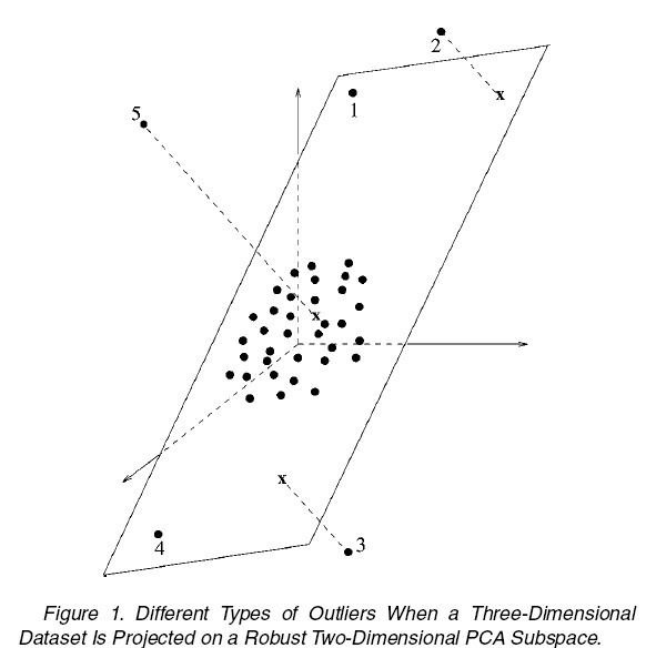
2. good leverage: far from regular points, but lie close to the true subspace, as point 1 and 4 in figure 1.

3. bad leverage: far from regular points, and also have a large orthogonal distance to the true subspace, as point 2 and 3 in figure 1.

4. orthogonal outliers: have a large orthogonal distance to the true subspace, but close to the regular points if projected into the true subspace, as point 5 in figure 1.

A diagnostic plot can be constructed to identify the types of each point as following:

1. On the horizontal axis, the robust score distance [math]\displaystyle{ SD_{i} }[/math] of each observation are plotted.

[math]\displaystyle{ SD_{i}=\sqrt{\sum_{j=1}^{k}\frac{t_{ij}^{2}}{l_{j}}} }[/math]

where the scores [math]\displaystyle{ t_{ij} }[/math] and [math]\displaystyle{ l_{j} }[/math]are obtained from step 3.

2. On the vertical axis, the orthogonal distance [math]\displaystyle{ OD_{i} }[/math] of each observation to the PCA subspace are plotted.

[math]\displaystyle{ OD_{i}=\left\| \mathbf{x}_{i}-\widehat{mu}-\mathbf{P}_{p,k}\mathbf{t}_{i}^{\prime} \right\| }[/math]

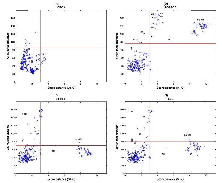
Then one can draw two cutoff lines (on horizontal and vertical axis respectively), and divide the diagnostic plot into four zones. Points fall into the lower-left zone are regular points, lower-right are good leverage points, upper-left are orthogonal outlying points, and upper-right are bad leverage points.

Example and Simulations

The performances of ROBPCA and the diagnostic plot are illustrated by some real data example and simulation studies. The comparison is carried out between ROBPCA and other four types of PCA: classical PCA (CPCA), RAPCA<ref name="HR">Reference</ref>, spherical PCA (SPHER) and ellipsoidal PCA (ELL)<ref>Locantore, N., Marron, J. S., Simpson, D. G., Tripoli, N., Zhang, J. T., and Cohen, K. L. Robust Principal Component Analysis for Functional Data. Test, 8:1-73, 1999</ref>, where the last three methods are also designed to be robust for high-dimensional data.

Examples

Glass data

The Glass dataset consists of 180 glass samples ([math]\displaystyle{ n=180 }[/math]), with 750 variables ([math]\displaystyle{ p=750 }[/math]).

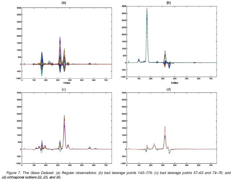
Perform ROBPCA on this dataset with the choice of [math]\displaystyle{ h=126=0.7n }[/math], and the dimensionality of the subspace [math]\displaystyle{ k=3 }[/math]. The diagnostic plot is shown as following. Clearly, ROBPCA distinguishes a small group of bad leverage points which all three other PCA methods fails to recognize. Moreover, through next figure, we can see ROBPCA identify the bad leverage points correctly.

Car data The car data contains 111 observations with p=11 characteristics measured for each car. The first 2 principle components are chosen since they account for 94% total variance (ROBPCA). The following figures show the diagnostic plots of ROBPCA and CPCA. Although the same set of outliers are detected, the group of bad leverage points from ROBPCA are converted into good leverage points for CPCA.

Simulations

In the simulation study, we generate 1000 samples of size n from the contamination model

[math]\displaystyle{ (1-\epsilon)F_{p}(0,\Sigma)+\epsilon F_{p}(\tilde{\mu},\tilde{\Sigma}) }[/math]

where [math]\displaystyle{ F_{p} }[/math] is p-variate Normal distribution or elliptical distribution.

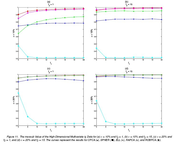
Different choices of [math]\displaystyle{ n,p,\epsilon,\Sigma,\tilde{\mu},\tilde{\Sigma} }[/math] are tried. The following tables and figures report some typical situations:

1. [math]\displaystyle{ \,n=100,p=4,\Sigma=diag(8,4,2,1),k=3 }[/math]

  (1a) [math]\displaystyle{ \,\epsilon=0 }[/math]: no comtamination
  
  (1b) [math]\displaystyle{ \,\epsilon }[/math]: 0.1 or 0.2
  
       [math]\displaystyle{ \tilde{\mu}=(0,0,0,f_{1})^{\prime},\tilde{\Sigma}=\Sigma/f_{2} }[/math]
      
       [math]\displaystyle{ f_{1}=6,8,10,\cdots,20 }[/math]
      
       [math]\displaystyle{ \,f_{2}=1,15 }[/math]

2. [math]\displaystyle{ n=50,p=100,\Sigma=diag(17,13.5,8,3,1,0.095,\cdots,0.001),k=5 }[/math]

  (2a) [math]\displaystyle{ \,\epsilon=0 }[/math]: no comtamination
  
  (2b) [math]\displaystyle{ \,\epsilon }[/math]: 0.1 or 0.2
  
       [math]\displaystyle{ \tilde{\mu}=(0,0,0,0,0,f_{1})^{\prime},\tilde{\Sigma}=\Sigma/f_{2} }[/math]
      
       [math]\displaystyle{ f_{1}=6,8,10,\cdots,20 }[/math]
      
       [math]\displaystyle{ \,f_{2}=1,15 }[/math]

For each simulation setting, the results of four methods are summarized as following:

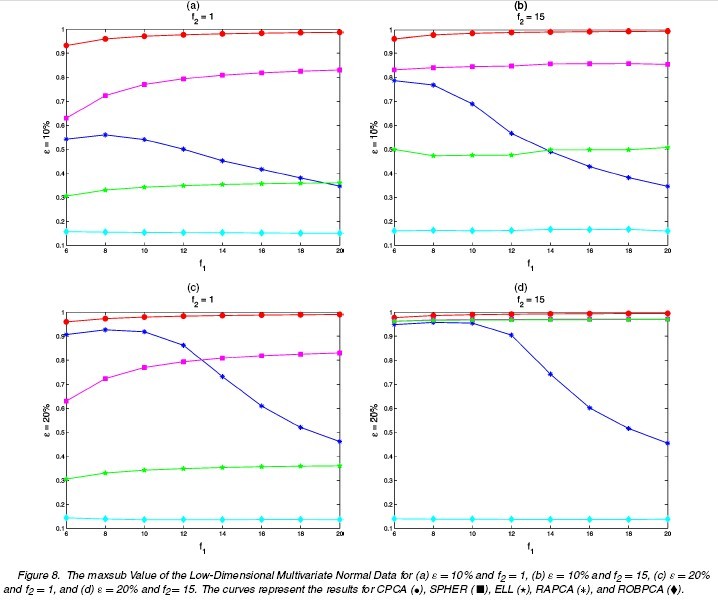
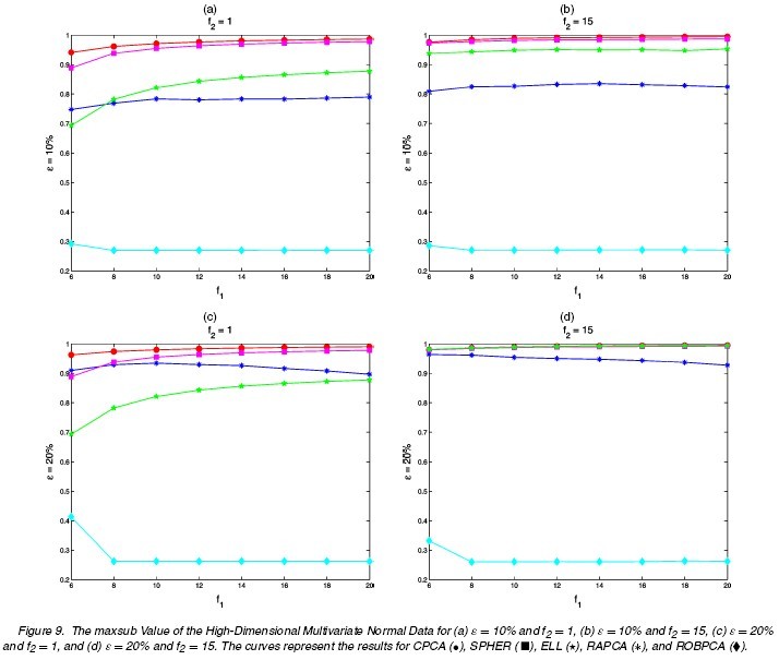
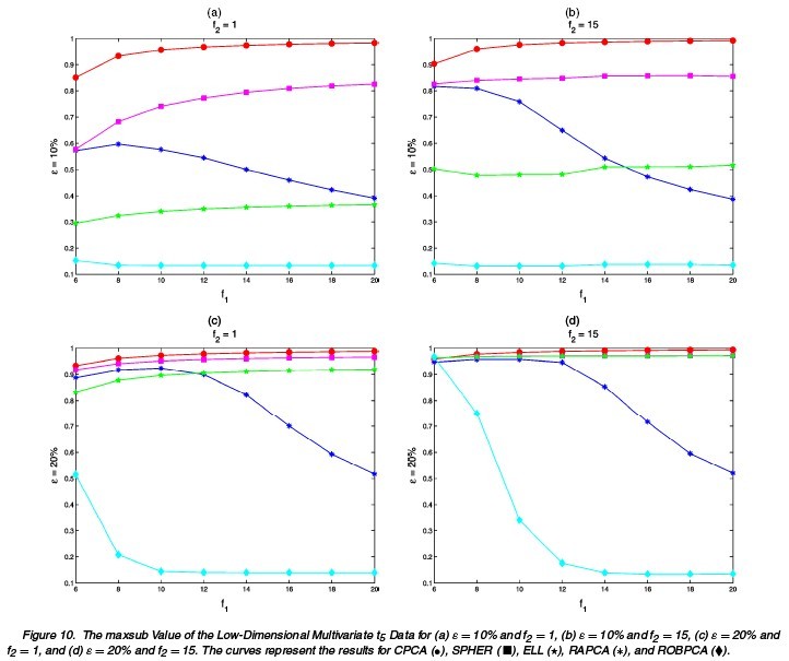
1. For each method, consider the maximal angle between the true subspace and estimated subspace<ref>Krzanowski, W. J. RBetween-Groups Comparison of Principal Components. Journal of the American Statistical Association, 74:703-707, 1979</ref>:

[math]\displaystyle{ maxsub=\frac{2}{\pi}arccos(\sqrt{\lambda_{k}}) }[/math]

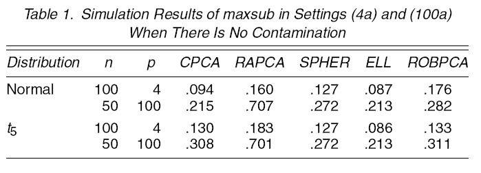
This is reported in table 1

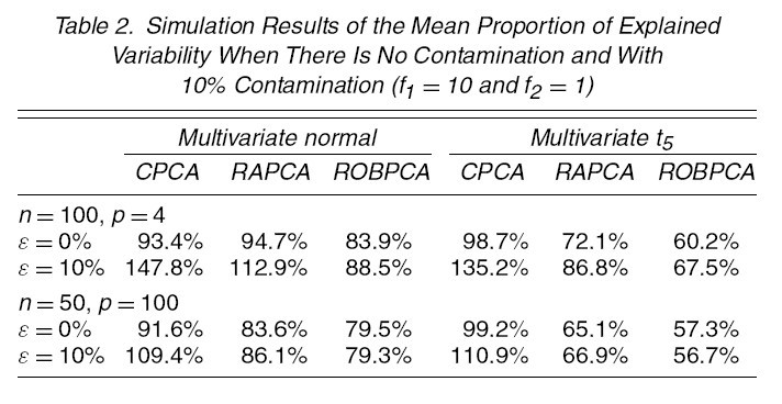
2. Consider the proportion of variability that is preserved by the estimated subspace. This is reported in table 2

3. Consider the mean squared error (MSE) for the k largest eigenvalues

[math]\displaystyle{ MSE(\widehat{\lambda}_{j})=\frac{1}{1000}\sum^{1000}_{l=1}(\widehat{\lambda}_{j}-\lambda_{j})^{2} }[/math]

The results for differnt settings are shown in the following figures.

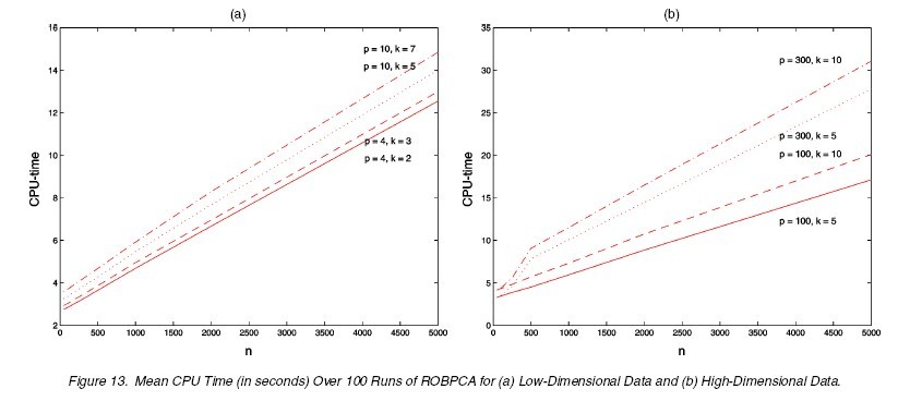
The last issue worth mentioning is the computation cost. The ROBPCA is slightly more computationaly expensive than other three methods compared above, but it is still acceptable. The following figure shows the mean CPU time in seconds over 100 runs for varying low-dimensional normal data

Reference

<references />