an HDP-HMM for Systems with State Persistence
Introduction
The Big Picture
Hidden Markov Model is one of the most effective and widely used probabilistic models for time series data. When there is not enough information available about the nature if the system, a serious limitation of this model is the needs to define the number of states for the model on prior (in other cases, like the problem of speech recognition, the number of states can be chosen based on the number of a subset of words in a dictionary). This number cannot be easily determined in real life applications. The usual way to define it is by a trying several different numbers of states and choose the one that gives the best results (trial and error approach). This limitation can be overcomed by types of probabilistic models called “Bayesian Nonparametric Models”. Bayesian Nonparametric Models approach this problem by defining distributions that can have infinite number of parameters. However, the assumption here is that even though the distribution could have infinite number of parameters, only finite number of them is required to explain the observed data.
A huge breakthrough in the possible applications of “Bayesian Nonparametric Methods” occurred after a paper published in 2005 by Yee Whye The, Michael I. Jordan, et.al. The title of the paper was “Hierarchical Dirichlet Processes (HDP)”. This paper describes a way to define a nonparametric Bayesian prior that allows atoms (which can be seen as components of mixture models) to be shared between groups of data (draws from mixture models). One application of this model was an extension to the Hidden Markov Model. The new model, which named HDP-HMM, allows the number of stats to be infinite.
The paper that I’m reviewing here proposes an augmented version of the HDP-HMM that solves the problem of state persistence. This problem also arises in the original Hidden Markov Model. The states in situations where this problem could occur have the tendency not to change their values, i.e. the transition probability to a new state is less than the probability of staying at the same state. The authors did not only provide a solution for this problem, but they also provided a full Bayesian treatment for it.
Speaker Diarization Problem
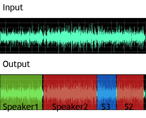
The task of segmenting or annotating an audio recording into different temporal segments where each segment corresponds to a specific event or speaker is called Speaker Diarization. One example of where Speaker Diarization could be useful is when analyzing a few minutes recorded audio from a radio broadcast. This few minutes could consist of commercials, intro music, a speech of the host, and a speech of the guest. The Speaker Diarization problem on such an audio recording could be defined as identifying speech and non-speech segments. Audio recording of meetings with known or unknown number of participants is another example the uses of Speaker Diarization. In this case the task is to answer the question of “who spoke when”. <ref>Tranter, S.E. and Reynolds, D.A., An Overview of Automatic Speaker Diarization Systems, 2006</ref>
The most common technique for solving the Speaker Diarization problem, which has also showed better results than others, is using Hidden Markov Models. In this setting, each speaker is associated with a specified state in the HMM. The transition among these stats represents the transition among speakers. However, a model like this suffers from a serious limitation. It requires the number of speakers to be known in advanced, which is needed to design the structure of the model.
The authors of this paper proposed a solution to the problem of Speaker Diarization on situations where a prior knowledge of the number of participants is unavailable. Their solution is based on a slightly modified version of an interesting Bayesian non-parametric model called “Hierarchical Dirichlet Process–Hidden Markov Model (HDP-HMM)”. The proposed modified version, which named “Sticky HDP-HMM”, imposes state persistence on the model.
A a possible solution to the question which asks:
There is a technique called blind source separation (BSS). In this approach we assume several speakers have spoken and they may have overlap. It means that in the same time two or more speakers may speak. This method is able to separate sources when we only have the mixture of the voices. So why don't we use this method? Why it is claimed HMM is better? The limitation of explained method is that it assumes only one speaker speaks at a time but BSS doesn't have this limitation.
One may say that BSS is based on the independent component analysis (ICA), which by itself depends upon the right selection of the type of nonlinearity. It will optimally distinguish different speakers, even if they are talking concurrently, just if we know the very type of kernel needed for ICA. However, Sticky HDP-HMM does not require making the choice of kernel, as it is built upon
Background
Nonparametric Bayesian Models
The Nonparametric Bayesian Models that we are considering in this discussion can be defined (informally) as follows. The word nonparametric does not mean that those models have no parameters, but in contrary it means that those models have infinite parameters spaces. And the fact that those models are Bayesian means that we are defining probability measures over them.
Dirichlet Process
Dirichlet Process is an example of Nonparametric Bayesian Models. It is a generalization of the Dirichlet Distribution, where the number of parameters can be infinite. The Dirichlet Distribution can be seen as a distribution over distributions of N outcomes. Thus, a draw from a Dirichlet Distribution is itself a probability distribution. Dirichlet Process has the same characteristic; it is a distribution over distributions, but the difference is that the outcomes N can grow and go to infinity. The DP is commonly used as a prior on the parameters of a mixture model of unknown complexity, resulting in a DPMM.
Dirichlet Distribution
Let [math]\displaystyle{ \theta = \{ \theta_1, \theta_2, ..., \theta_m\} }[/math] such that [math]\displaystyle{ \theta }[/math]~[math]\displaystyle{ Dirichlet(\alpha_1, \alpha_2, ..., \alpha_m) }[/math], then the distribution is defined by: [math]\displaystyle{ \, P(\theta_1, \theta_2, \theta_3 ,...,\theta_m) = \frac{\Gamma (\sum_k \alpha_k)}{\prod_k \Gamma(\alpha_k)} \prod_{k=1}^{m} \theta_k^{\alpha_k - 1} }[/math]. As an example, the Beta distribution is the special case of Dirichlet distribution for two dimensions. In fact, the Dirichlet distribution is a "distribution over distribution".
A Dirichlet process [math]\displaystyle{ DP(H,\alpha) }[/math] is defined using two parameters. The first parameter, [math]\displaystyle{ H }[/math], is a base distribution. This parameter can be considered as the mean of the Dirichlet Process. The second parameter, [math]\displaystyle{ \alpha }[/math], is called the concentration parameter.
As described above, a draw from a Dirichlet process is discrete probability measure, regardless of wither the base distribution is discrete or continuous. This fact is one of the most important properties of Dirichlet Process; it assures that draws from the Dirichlet Process can be repeated.
A stick breaking construction of the Dirichlet Process was introduced in (Sethuraman, 1994), as follows:
[math]\displaystyle{ \, \beta_k = \beta_{‘}^{k} \prod_{l=1}^{k-1}(1-\beta_{l}^{'}) }[/math]
[math]\displaystyle{ \, \beta_{l}^{'} }[/math]~[math]\displaystyle{ \, Beta(1,\gamma) }[/math]
[math]\displaystyle{ \, G_o = \sum_{k=1}^{\infty} \beta_k \delta(\theta - \theta_k) }[/math]
[math]\displaystyle{ \, \theta_k }[/math]~[math]\displaystyle{ \, H }[/math]
This specific construction is usually denoted by: [math]\displaystyle{ \, \beta }[/math]~[math]\displaystyle{ \, GEM(\gamma) }[/math]
Hierarchical Dirichlet Processes
The hierarchical Dirichlet process (HDP) (Teh et al.,2006) extends the DP to cases in which groups of data are produced by related, yet unique, generative processes. Two Dirichlet Process can be used together in a recursion way such that a draw from the first one uses as the base distribution of the second one. Formally,
[math]\displaystyle{ \, G }[/math] ~ [math]\displaystyle{ \, DP(\alpha, G_0) }[/math]
[math]\displaystyle{ \, G_0 }[/math] ~ [math]\displaystyle{ \, DP(\gamma, H) }[/math].
Doing so would allow us to share atoms. The analogy here is that we are modeling a grouped of data and each group of them was modeled using a mixture model.
Sticky HDP-HMM
HMM
One way to look at the HMM is as a doubly stochastic Markov chain. It consists of a set of state variables that are usually defined as a multinomial random variable. These variables are linked together by a transition matrix. The observations are independent of each other and conditioned only on the state variable that they are belonging to.
HDP-HMM
In [Ref::Teh05], an extension to the HMM was introduced. This extension allows the number of stats to be infinite using the Hierarchical Dirichlet Process. Their extension works as follows. Let [math]\displaystyle{ \, S_t }[/math] denote the state of the HMM at time t. As this variable follows a Markov chain, its value is going to be drawn from a distribution that is conditioned on the value of the previous state [math]\displaystyle{ \, S_t }[/math] ~ [math]\displaystyle{ \, \pi_{S_t-1} }[/math]. The value of this variable, [math]\displaystyle{ \, S_t }[/math], is then used to draw an observation, i.e [math]\displaystyle{ \, y }[/math] ~ [math]\displaystyle{ \, F(\theta_{S_t})) }[/math]. Now by defining [math]\displaystyle{ \, \pi_{k} }[/math] as: [math]\displaystyle{ \, \pi_{k} }[/math] ~ [math]\displaystyle{ \, HDP(.) }[/math]. We can have infinite shared states among all the stat variables. <ref> Teh, 2055. Hierarchical Dirichlet Processes </ref>

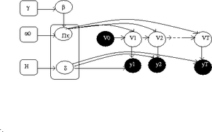
Here is a sample figure of HDP-HMM taken from <ref>Teh YW, Jordan MI, Beal MJ and Blei DM , Hierarchical Dirichlet Processes, 2005</ref>
In the figure, we have a sequence of multinomial variables [math]\displaystyle{ (v_1,v_2,\dots,v_T) }[/math] that are attached to a sequence of observations [math]\displaystyle{ (y_1,y_2,\dots,y_T) }[/math]. These observations are drawn independently conditioned on the [math]\displaystyle{ v_i }[/math]. The set of finite mixture models in the HMM is replaced by a hierarchical Dirichlet process.
Sticky HDP-HMM
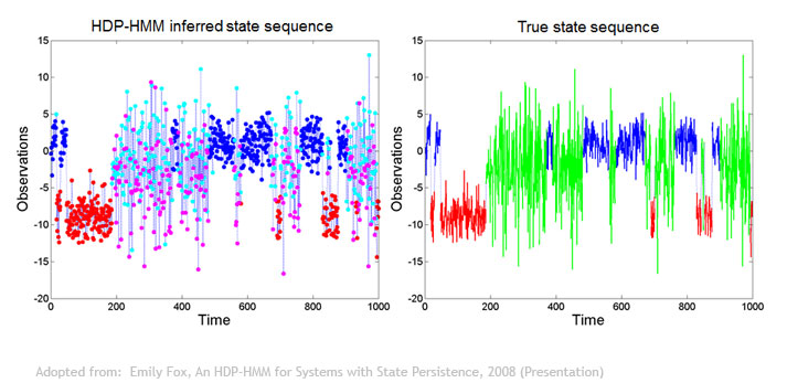
Although substituting the distribution of [math]\displaystyle{ \, \pi_{k} }[/math] by a hierarchal nonparametric Bayesian prior provided us with a way to have infinite number of states, the problem of states persistence, which was described above, is still existed. It Is getting even more serious under this setting as the HDP would generate more states to explain all the transitions, so instead of having a larger probability to stay at the same state, a new redundant states would be generated. The next figure shows an example of this problem. The right side of the figure shows the true state sequence in which there are only three states that explain the observed data (labeled using different colors). The right left side, on the other hand, shows the inferred state sequence for the same data using HDP-HMM. In this case, the model spited some of the true states into more than one state and rapidly switches between them.
To overcome this problem, the authors proposed a modification to the transition distribution as follows:
[math]\displaystyle{ \, \pi_j }[/math] ~ [math]\displaystyle{ \, DP( \alpha+ k, \frac{\alpha \beta + k \delta_j}{\alpha + j}) }[/math]
This main new term [math]\displaystyle{ \, k \delta_j }[/math] adds the amount k to the jth component of the base distribution so that it increases the prior probability of self-transition from state j to itself. Note that the original HDP-HMM can be restored from this model by setting k = 0. {{
Template:namespace detect
| type = style | image = | imageright = | style = | textstyle = | text = This article may require cleanup to meet Wikicoursenote's quality standards. The specific problem is: I think it is necessary to explain how HDP-HMM is used for the original voice recognition problem and provide more experiments.. Please improve this article if you can. (November 2011) | small = | smallimage = | smallimageright = | smalltext = }}
References
<references/>

