stat841f11

STAT 441/841 / CM 463/763 - Tuesday, 2011/09/20

Wiki Course Notes

Students will need to contribute to the wiki for 20% of their grade. Access via wikicoursenote.com Go to editor sign-up, and use your UW userid for your account name, and use your UW email.

primary (10%) Post a draft of lecture notes within 48 hours. You will need to do this 1 or 2 times, depending on class size.

secondary (10%) Make improvements to the notes for at least 60% of the lectures. More than half of your contributions should be technical rather than editorial. There will be a spreadsheet where students can indicate what they've done and when. The instructor will conduct random spot checks to ensure that students have contributed what they claim.

Classification (Lecture: Sep. 20, 2011)

Introduction

Machine learning (ML) methodology in general is an artificial intelligence approach to establish and train a model to recognize the pattern or underlying mapping of a system based on a set of training examples consisting of input and output patterns. Unlike in classical statistics where inference is made from small datasets, machine learning involves drawing inference from an overwhelming amount of data that could not be reasonably parsed by manpower.

In machine learning, pattern recognition is the assignment of some sort of output value (or label) to a given input value (or instance), according to some specific algorithm. The approach of using examples to produce the output labels is known as learning methodology. When the underlying function from inputs to outputs exists, it is referred to as the target function. The estimate of the target function which is learnt or output by the learning algorithm is known as the solution of learning problem. In case of classification this function is referred to as the decision function.

In the broadest sense, any method that incorporates information from training samples in the design of a classifier employs learning. Learning tasks can be classified along different dimensions. One important dimension is the distinction between supervised and unsupervised learning. In supervised learning a category label for each pattern in the training set is provided. The trained system will then generalize to new data samples. In unsupervised learning , on the other hand, training data has not been labeled, and the system forms clusters or natural grouping of input patterns based on some sort of measure of similarity and it can then be used to determine the correct output value for new data instances.

The first category is known as pattern classification and the second one as clustering. Pattern classification is the main focus in this course.

Classification problem formulation : Suppose that we are given n observations. Each observation consists of a pair: a vector ${\mathbf{x}}_i\subset {\mathbb{R}}^d,i=1,...,n$, and the associated label $y_i$. Where ${\mathbf{x}}_i=(x_{i1},x_{i2},...x_{id})\in \mathcal{X}\subset {\mathbb{R}}^d$ and $Y_i$ belongs to some finite set $\mathcal{Y}$.

The classification task is now looking for a function $f:{\mathbf{x}}_i\mapsto y$ which maps the input data points to a target value (i.e. class label). Function $f(\mathbf{x},\theta )$ is defined by a set of parametrs $\theta$ and the goal is to train the classifier in a way that among all possible mappings with different parameters the obtained decision boundary gives the minimum classification error.

Definitions

The true error rate for classifier $h$ is the error with respect to the unknown underlying distribution when predicting a discrete random variable Y from a given input X.

$L(h)=P(h(X)\ne Y)$

The empirical error rate is the error of our classification function $h(x)$ on a given dataset with known outputs (e.g. training data, test data)

${\hat{L}}_n(h)=(1/n)\sum _{i=1}^n\mathbf{I}(h(X_i)\ne Y_i)$ where h is a clssifier and $\mathbf{I}()$ is an indicator function. The indicator function is defined by

$\mathbf{I}(x)=\{\begin{array}{ll}1& \text{if }x\text{ is true}\\ 0& \text{if }x\text{ is false}\end{array}$

So in this case, $\mathbf{I}(h(X_i)\ne Y_i)=\{\begin{array}{ll}1& \text{if }h(X_i)\ne Y_i\text{ (i.e. misclassification)}\\ 0& \text{if }h(X_i)=Y_i\text{ (i.e. classified properly)}\end{array}$

For example, suppose we have 100 new data points with known (true) labels

$X_1...X_{100}$ $y_1...y_{100}$

To calculate the empirical error, we count how many times our function $h(X)$ classifies incorrectly (does not match $y$) and divide by n=100.

Bayes Classifier

The principle of the Bayes Classifier is to calculate the posterior probability of a given object from its prior probability via Bayes' Rule, and then assign the object to the class with the largest posterior probability<ref> http://www.wikicoursenote.com/wiki/Stat841#Bayes_Classifier </ref>.

First recall Bayes' Rule, in the format $P(Y|X)=\frac{P(X|Y)P(Y)}{P(X)}$

P(Y|X)  : posterior , probability of $Y$ given $X$

P(X|Y)  : likelihood, probability of $X$ being generated by $Y$

P(Y)  : prior, probability of $Y$ being selected

P(X)  : marginal, probability of obtaining $X$

We will start with the simplest case: $\mathcal{Y}=\{0,1\}$

$r(x)=P(Y=1|X=x)=\frac{P(X=x|Y=1)P(Y=1)}{P(X=x)}=\frac{P(X=x|Y=1)P(Y=1)}{P(X=x|Y=1)P(Y=1)+P(X=x|Y=0)P(Y=0)}$

Bayes' rule can be approached by computing either one of the following:

1) The posterior: $P(Y=1|X=x)$ and $P(Y=0|X=x)$

2) The likelihood: $P(X=x|Y=1)$ and $P(X=x|Y=0)$

The former reflects a Bayesian approach. The Bayesian approach uses previous beliefs and observed data (e.g., the random variable $X$) to determine the probability distribution of the parameter of interest (e.g., the random variable $Y$). The probability, according to Bayesians, is a degree of belief in the parameter of interest taking on a particular value (e.g., $Y=1$), given a particular observation (e.g., $X=x$). Historically, the difficulty in this approach lies with determining the posterior distribution. However, more recent methods such as Markov Chain Monte Carlo (MCMC) allow the Bayesian approach to be implemented <ref name="PCAustin">P. C. Austin, C. D. Naylor, and J. V. Tu, "A comparison of a Bayesian vs. a frequentist method for profiling hospital performance," Journal of Evaluation in Clinical Practice, 2001</ref>.

The latter reflects a Frequentist approach. The Frequentist approach assumes that the probability distribution (including the mean, variance, etc.) is fixed for the parameter of interest (e.g., the variable $Y$, which is not random). The observed data (e.g., the random variable $X$) is simply a sampling of a far larger population of possible observations. Thus, a certain repeatability or frequency is expected in the observed data. If it were possible to make an infinite number of observations, then the true probability distribution of the parameter of interest can be found. In general, frequentists use a technique called hypothesis testing to compare a null hypothesis (e.g. an assumption that the mean of the probability distribution is ${\mu }_0$) to an alternative hypothesis (e.g. assuming that the mean of the probability distribution is larger than ${\mu }_0$) <ref name="PCAustin"/>. For more information on hypothesis testing see <ref>R. Levy, "Frequency hypothesis testing, and contingency tables" class notes for LING251, Department of Linguistics, University of California, 2007. Available: http://idiom.ucsd.edu/~rlevy/lign251/fall2007/lecture_8.pdf </ref>.

There was some class discussion on which approach should be used. Both the ease of computation and the validity of both approaches were discussed. A main point that was brought up in class is that Frequentists consider X to be a random variable, but they do not consider Y to be a random variable because it has to take on one of the values from a fixed set (in the above case it would be either 0 or 1 and there is only one correct label for a given value X=x). Thus, from a Frequentist's perspective it does not make sense to talk about the probability of Y. This is actually a grey area and sometimes Bayesians and Frequentists use each others' approaches. So using Bayes' rule doesn't necessarily mean you're a Bayesian. Overall, the question remains unresolved.

The Bayes Classifier uses $P(Y=1|X=x)$

$P(Y=1|X=x)=\frac{P(X=x|Y=1)P(Y=1)}{P(X=x|Y=1)P(Y=1)+P(X=x|Y=0)P(Y=0)}$

P(Y=1) : the prior, based on belief/evidence beforehand

denominator : marginalized by summation

$h(x)=\{\begin{array}{l}1\hat{r}(x)>1/2\\ 0otherwise\end{array}$

The set $\mathcal{D}(h)=\{x:P(Y=1|X=x)=P(Y=0|X=x)...\}$

which defines a decision boundary.

$h^{\ast }(x)=\{\begin{array}{l}1ifP(Y=1|X=x)>P(Y=0|X=x)\\ 0otherwise\end{array}$

Theorem: The Bayes Classifier is optimal, i.e., if $h$ is any other classification rule, then $L(h^{\ast })<=L(h)$

Proof: Consider any classifier $h$. We can express the error rate as

$P(\{h(X)\ne Y\})=E_{X,Y}[{\mathbf{1}}_{\{h(X)\ne Y\}}]=E_X[E_Y[{\mathbf{1}}_{\{h(X)\ne Y\}}|X]]$

To minimize this last expression, it suffices to minimize the inner expectation. Expanding this expectation:

$E_Y[{\mathbf{1}}_{\{h(X)\ne Y\}}|X]=\sum _{y\in Supp(Y)}P(h(X)\ne y|X){\mathbf{1}}_{\{h(X)\ne y\}}$

which, in the two-class case, simplifies to

$=P(h(X)\ne 0|X){\mathbf{1}}_{\{h(X)\ne 0\}}+P(h(X)\ne 1|X){\mathbf{1}}_{\{h(X)\ne 1\}}$

$=r(X){\mathbf{1}}_{\{h(X)\ne 0\}}+(1-r(X)){\mathbf{1}}_{\{h(X)\ne 1\}}$

where $r(x)$ is defined as above. We should 'choose' h(X) to equal the label that minimizes the sum. Consider if $r(X)>1/2$, then $r(X)>1-r(X)$ so we should let $h(X)=1$ to minimize the sum. Thus the Bayes classifier is the optimal classifier.

Why then do we need other classification methods? Because X densities are often/typically unknown. I.e., $f_k(x)$ and/or ${\pi }_k$ unknown.

$P(Y=k|X=x)=\frac{P(X=x|Y=k)P(Y=k)}{P(X=x)}=\frac{f_k(x){\pi }_k}{\sum _k{f}_k(x){\pi }_k}$ f_k(x) is referred to as the class conditional distribution (~likelihood).

Therefore, we rely on some data to estimate quantities.

Three Main Approaches

1. Empirical Risk Minimization: Choose a set of classifiers H (e.g., line, neural network) and find $h^{\ast }\in H$ that minimizes (some estimate of) L(h).

2. Regression: Find an estimate ($\hat{r}$) of function $r$ and define $h(x)=\{\begin{array}{l}1\hat{r}(x)>1/2\\ 0otherwise\end{array}$

The $1/2$ in the expression above is a threshold set for the regression prediction output.

In general regression refers to finding a continuous, real valued y. The problem here is more difficult, because of the restricted domain (y is a set of discrete label values).

3. Density Estimation: Estimate $P(X=x|Y=0)$ from $X_i$'s for which $Y_i=0$ Estimate $P(X=x|Y=1)$ from $X_i$'s for which $Y_i=1$ and let $P(Y=?)=(1/n)\sum _{i=1}^n{Y}_i$

Define $\hat{r}(x)=\hat{P}(Y=1|X=x)$ and $h(x)=\{\begin{array}{l}1\hat{r}(x)>1/2\\ 0otherwise\end{array}$

It is possible that there may not be enough data to estimate from for density estimation. But the main problem lies with high dimensional spaces, as the estimation results may not be good (high error rate) and sometimes even infeasible. The term curse of dimensionality was coined by Bellman <ref>R. E. Bellman, Dynamic Programming. Princeton University Press, 1957</ref> to describe this problem.

As the dimension of the space goes up, the learning requirements go up exponentially.

To Learn more about methods for handling high-dimensional data <ref> https://docs.google.com/viewer?url=http%3A%2F%2Fwww.bios.unc.edu%2F~dzeng%2FBIOS740%2Flecture_notes.pdf</ref>

The simplest approach to classification is to use the third approach.

Multi-Class Classification

Generalize to case Y takes on k>2 values.

Theorem: $Y\in \mathcal{Y}=\{1,2,...,k\}$ optimal rule

$h^{\ast }(x)=argma{x}_{k}P(Y=k|X=x)$

where $P(Y=k|X=x)=\frac{f_k(x){\pi }_k}{\sum _r{f}_r{\pi }_r}$

Examples of Classification

• Face detection in images.
• Medical diagnosis.
• Detecting credit card fraud (fraudulent or legitimate).
• Speech recognition.
• Handwriting recognition.

LDA and QDA

Discriminant function analysis finds features that best allow discrimination between two or more classes. The approach is similar to analysis of Variance (ANOVA) in that discriminant function analysis looks at the mean values to determine if two or more classes are very different and should be separated. Once the discriminant functions (that separate two or more classes) have been determined, new data points can be classified (i.e. placed in one of the classes) based on the discriminant functions <ref> StatSoft, Inc. (2011). Electronic Statistics Textbook. [Online]. Available: http://www.statsoft.com/textbook/discriminant-function-analysis/. </ref>. Linear discriminant analysis (LDA) and Quadratic discriminant analysis (QDA) are methods of discriminant analysis that are best applied to linearly and quadradically separable classes, respectively. Fisher discriminant analysis (FDA) another method of discriminant analysis that is different from linear discriminant analysis, but oftentimes both terms are used interchangeably.

LDA

The simplest method is to use approach 3 (above) and assume a parametric model for densities. Assume class conditional is Gaussian.

$\mathcal{Y}=\{0,1\}$ assumed (i.e., 2 labels)

$h(x)=\{\begin{array}{l}1P(Y=1|X=x)>P(Y=0|X=x)\\ 0otherwise\end{array}$

$P(Y=1|X=x)=\frac{f_1(x){\pi }_1}{\sum _k{f}_k{\pi }_k}$ (denom = P(x))

1) Assume Gaussian distributions

$f_k(x)=\frac{1}{(2\pi {)}^{d/2}|{\mathrm{\Sigma }}_k{|}^{1/2}}\text{exp}(-\frac{1}{2}(\mathbf{x}\mathbf{-}{\mu }_{\mathbf{k}}){\mathrm{\Sigma }}_k^{-1}(\mathbf{x}\mathbf{-}{\mu }_{\mathbf{k}}))$

must compare $\frac{f_1(x){\pi }_1}{p(x)}$ with $\frac{f_0(x){\pi }_0}{p(x)}$ Note that the p(x) denom can be ignored: $f_1(x){\pi }_1$ with $f_0(x){\pi }_0$

To find the decision boundary, set $f_1(x){\pi }_1=f_0(x){\pi }_0$

$\frac{1}{(2\pi {)}^{d/2}|{\mathrm{\Sigma }}_1{|}^{1/2}}exp(-\frac{1}{2}(\mathbf{x}\mathbf{-}{\mu }_{\mathbf{1}}){\mathrm{\Sigma }}_1^{-1}(\mathbf{x}\mathbf{-}{\mu }_{\mathbf{1}})){\pi }_1=\frac{1}{(2\pi {)}^{d/2}|{\mathrm{\Sigma }}_0{|}^{1/2}}exp(-\frac{1}{2}(\mathbf{x}\mathbf{-}{\mu }_{\mathbf{0}}){\mathrm{\Sigma }}_0^{-1}(\mathbf{x}\mathbf{-}{\mu }_{\mathbf{0}})){\pi }_0$

2) Assume ${\mathrm{\Sigma }}_1={\mathrm{\Sigma }}_0$, we can use $\mathrm{\Sigma }={\mathrm{\Sigma }}_0={\mathrm{\Sigma }}_1$.

$\frac{1}{(2\pi {)}^{d/2}|\mathrm{\Sigma }{|}^{1/2}}exp(-\frac{1}{2}(\mathbf{x}\mathbf{-}{\mu }_{\mathbf{1}}){\mathrm{\Sigma }}^{-1}(\mathbf{x}\mathbf{-}{\mu }_{\mathbf{1}})){\pi }_1=\frac{1}{(2\pi {)}^{d/2}|\mathrm{\Sigma }{|}^{1/2}}exp(-\frac{1}{2}(\mathbf{x}\mathbf{-}{\mu }_{\mathbf{0}}){\mathrm{\Sigma }}^{-1}(\mathbf{x}\mathbf{-}{\mu }_{\mathbf{0}})){\pi }_0$

3) Cancel $(2\pi {)}^{-d/2}|\mathrm{\Sigma }{|}^{-1/2}$ from both sides.

$exp(-\frac{1}{2}(\mathbf{x}\mathbf{-}{\mu }_{\mathbf{1}}){\mathrm{\Sigma }}^{-1}(\mathbf{x}\mathbf{-}{\mu }_{\mathbf{1}})){\pi }_1=exp(-\frac{1}{2}(\mathbf{x}\mathbf{-}{\mu }_{\mathbf{0}}){\mathrm{\Sigma }}^{-1}(\mathbf{x}\mathbf{-}{\mu }_{\mathbf{0}})){\pi }_0$

4) Take log of both sides.

$-\frac{1}{2}(\mathbf{x}\mathbf{-}{\mu }_{\mathbf{1}}){\mathrm{\Sigma }}^{-1}(\mathbf{x}\mathbf{-}{\mu }_{\mathbf{1}}))+\text{log}({\pi }_1)=-\frac{1}{2}(\mathbf{x}\mathbf{-}{\mu }_{\mathbf{0}}){\mathrm{\Sigma }}^{-1}(\mathbf{x}\mathbf{-}{\mu }_{\mathbf{0}}))+\text{log}({\pi }_0)$

5) Subtract one side from both sides, leaving zero on one side.

$-\frac{1}{2}(\mathbf{x}\mathbf{-}{\mu }_{\mathbf{1}}{)}^T{\mathrm{\Sigma }}^{-1}(\mathbf{x}\mathbf{-}{\mu }_{\mathbf{1}})+\text{log}({\pi }_1)-[-\frac{1}{2}(\mathbf{x}\mathbf{-}{\mu }_{\mathbf{0}}{)}^T{\mathrm{\Sigma }}^{-1}(\mathbf{x}\mathbf{-}{\mu }_{\mathbf{0}})+\text{log}({\pi }_0)]=0$

$\frac{1}{2}[-{\mathbf{x}}^T{\mathrm{\Sigma }}^{-1}{\mathbf{x}\mathbf{-}{\mu }_{\mathbf{1}}}^T{\mathrm{\Sigma }}^{-1}{\mu }_{\mathbf{1}}+2{{\mu }_{\mathbf{1}}}^T{\mathrm{\Sigma }}^{-1}\mathbf{x}+{\mathbf{x}}^T{\mathrm{\Sigma }}^{-1}\mathbf{x}+{{\mu }_{\mathbf{0}}}^T{\mathrm{\Sigma }}^{-1}{\mu }_{\mathbf{0}}-2{{\mu }_{\mathbf{0}}}^T{\mathrm{\Sigma }}^{-1}\mathbf{x}]+\text{log}(\frac{{\pi }_1}{{\pi }_0})=0$

Cancelling out the terms quadratic in $\mathbf{x}$ and rearranging results in

$\frac{1}{2}[-{{\mu }_{\mathbf{1}}}^T{\mathrm{\Sigma }}^{-1}{\mu }_{\mathbf{1}}+{{\mu }_{\mathbf{0}}}^T{\mathrm{\Sigma }}^{-1}{\mu }_{\mathbf{0}}+(2{{\mu }_{\mathbf{1}}}^T{\mathrm{\Sigma }}^{-1}-2{{\mu }_{\mathbf{0}}}^T{\mathrm{\Sigma }}^{-1})\mathbf{x}]+\text{log}(\frac{{\pi }_1}{{\pi }_0})=0$

We can see that the first pair of terms is constant, and the second pair is linear in x. Therefore, we end up with something of the form $ax+b=0$. For more about LDA <ref>http://sites.stat.psu.edu/~jiali/course/stat597e/notes2/lda.pdf</ref>

LDA and QDA Continued (Lecture: Sep. 22, 2011)

If we relax assumption 2 (i.e. ${\mathrm{\Sigma }}_1\ne {\mathrm{\Sigma }}_0$) then we get a quadratic equation that can be written as $x^{T}ax+bx+c=0$

Generalizing LDA and QDA

Theorem:

Suppose that $Y\in \{1,\dots ,K\}$, if $f_k(\mathbf{x})=Pr(X=\mathbf{x}|Y=k)$ is Gaussian. The Bayes Classifier is

$h^{\ast }(\mathbf{x})=\arg \underset{k}{max}{\delta }_k(\mathbf{x})$

Where

${\delta }_k(\mathbf{x})=-\frac{1}{2}log(|{\mathrm{\Sigma }}_k|)-\frac{1}{2}(\mathbf{x}-{\mathit{\mu }}_k{)}^{\mathrm{\top }}{\mathrm{\Sigma }}_k^{-1}(\mathbf{x}-{\mathit{\mu }}_k)+log({\pi }_k)$

When the Gaussian variances are equal ${\mathrm{\Sigma }}_1={\mathrm{\Sigma }}_0$ (e.g. LDA), then

${\delta }_k(\mathbf{x})={\mathbf{x}}^{\mathrm{\top }}{\mathrm{\Sigma }}^{-1}{\mathit{\mu }}_k-\frac{1}{2}{\mathit{\mu }}_k^{\mathrm{\top }}{\mathrm{\Sigma }}^{-1}{\mathit{\mu }}_k+log({\pi }_k)$

(To compute this, we need to calculate the value of $\delta$ for each class, and then take the one with the max. value).

In practice

We estimate the prior to be the chance that a random item from the collection belongs to class k, e.g.

$\widehat{{\pi }_k}=\widehat{Pr}(y=k)=\frac{n_k}{n}$

The mean to be the average item in set k, e.g.

$\widehat{{\mu }_k}=\frac{1}{n_k}\sum _{i:y_i=k}{x}_i$

and calculate the covariance of each class e.g.

$\widehat{{\mathrm{\Sigma }}_k}=\frac{1}{n_k}\sum _{i:y_i=k}(x_i-\widehat{{\mu }_k})(x_i-\widehat{{\mu }_k}{)}^{\mathrm{\top }}$

If we wish to use LDA we must calculate a common covariance, so we average all the covariances e.g.

$\mathrm{\Sigma }=\frac{\sum _{r=1}^k(n_r{\mathrm{\Sigma }}_r)}{\sum _{r=1}^k{n}_r}$

Where: $n_r$ is the number of data points in class $r$, ${\mathrm{\Sigma }}_r$ is the covariance of class $r$, $n$ is the total number of data points, and $k$ is the number of classes.

Computation

For QDA we need to calculate: ${\delta }_k(\mathbf{x})=-\frac{1}{2}log(|{\mathrm{\Sigma }}_k|)-\frac{1}{2}(\mathbf{x}-{\mathit{\mu }}_k{)}^{\mathrm{\top }}{\mathrm{\Sigma }}_k^{-1}(\mathbf{x}-{\mathit{\mu }}_k)+log({\pi }_k)$

Lets first consider when ${\mathrm{\Sigma }}_k=I,\mathrm{\forall }k$. This is the case where each distribution is spherical, around the mean point.

Case 1

When ${\mathrm{\Sigma }}_k=I$

We have:

${\delta }_k=-\frac{1}{2}log(|I|)-\frac{1}{2}(\mathbf{x}-{\mathit{\mu }}_k{)}^{\mathrm{\top }}I(\mathbf{x}-{\mathit{\mu }}_k)+log({\pi }_k)$

but $\log (|I|)=\log (1)=0$

and $(\mathbf{x}-{\mathit{\mu }}_k{)}^{\mathrm{\top }}I(\mathbf{x}-{\mathit{\mu }}_k)=(\mathbf{x}-{\mathit{\mu }}_k{)}^{\mathrm{\top }}(\mathbf{x}-{\mathit{\mu }}_k)$ is the squared Euclidean distance between two points $\mathbf{x}$ and ${\mathit{\mu }}_k$

Thus in this condition, a new point can be classified by its distance away from the center of a class, adjusted by some prior.

Further, for two-class problem with equal prior, the discriminating function would be the bisector of the 2-class's means.

Case 2

When ${\mathrm{\Sigma }}_k\ne I$

Using the Singular Value Decomposition (SVD) of ${\mathrm{\Sigma }}_k$ we get ${\mathrm{\Sigma }}_k=U_k{S}_k{V}_k^{\mathrm{\top }}$. In particular, $U_k$ is a collection of eigenvectors of ${\mathrm{\Sigma }}_k{\mathrm{\Sigma }}_k^{\ast }$, and $V_k$ is a collection of eigenvectors of ${\mathrm{\Sigma }}_k^{\ast }{\mathrm{\Sigma }}_k$. Since ${\mathrm{\Sigma }}_k$ is a symmetric matrix<ref> http://en.wikipedia.org/wiki/Covariance_matrix#Properties </ref>, ${\mathrm{\Sigma }}_k={\mathrm{\Sigma }}_k^{\ast }$, so we have ${\mathrm{\Sigma }}_k=U_k{S}_k{U}_k^{\mathrm{\top }}$.

For ${\delta }_k$, the second term becomes what is also known as the Mahalanobis distance <ref>P. C. Mahalanobis, "On The Generalised Distance in Statistics," Proceedings of the National Institute of Sciences of India, 1936</ref> :

$\begin{array}{rl}(\mathbf{x}-{\mathit{\mu }}_k{)}^{\mathrm{\top }}{\mathrm{\Sigma }}_k^{-1}(\mathbf{x}-{\mathit{\mu }}_k)& =(\mathbf{x}-{\mathit{\mu }}_k{)}^{\mathrm{\top }}{U}_k{S}_k^{-1}{U}_k^T(\mathbf{x}-{\mathit{\mu }}_k)\\ & =(U_k^{\mathrm{\top }}\mathbf{x}-U_k^{\mathrm{\top }}{\mathit{\mu }}_k{)}^{\mathrm{\top }}{S}_k^{-1}(U_k^{\mathrm{\top }}\mathbf{x}-U_k^{\mathrm{\top }}{\mathit{\mu }}_k)\\ & =(U_k^{\mathrm{\top }}\mathbf{x}-U_k^{\mathrm{\top }}{\mathit{\mu }}_k{)}^{\mathrm{\top }}{S}_k^{-\frac{1}{2}}{S}_k^{-\frac{1}{2}}(U_k^{\mathrm{\top }}\mathbf{x}-U_k^{\mathrm{\top }}{\mathit{\mu }}_k)\\ & =(S_k^{-\frac{1}{2}}{U}_k^{\mathrm{\top }}\mathbf{x}-S_k^{-\frac{1}{2}}{U}_k^{\mathrm{\top }}{\mathit{\mu }}_k{)}^{\mathrm{\top }}I(S_k^{-\frac{1}{2}}{U}_k^{\mathrm{\top }}\mathbf{x}-S_k^{-\frac{1}{2}}{U}_k^{\mathrm{\top }}{\mathit{\mu }}_k)\\ & =(S_k^{-\frac{1}{2}}{U}_k^{\mathrm{\top }}\mathbf{x}-S_k^{-\frac{1}{2}}{U}_k^{\mathrm{\top }}{\mathit{\mu }}_k{)}^{\mathrm{\top }}(S_k^{-\frac{1}{2}}{U}_k^{\mathrm{\top }}\mathbf{x}-S_k^{-\frac{1}{2}}{U}_k^{\mathrm{\top }}{\mathit{\mu }}_k)\end{array}$

If we think of $S_k^{-\frac{1}{2}}{U}_k^{\mathrm{\top }}$ as a linear transformation that takes points in class $k$ and distributes them spherically around a point, like in case 1. Thus when we are given a new point, we can apply the modified ${\delta }_k$ values to calculate $h^{\ast }(x)$. After applying the singular value decomposition, ${\mathrm{\Sigma }}_k^{-1}$ is considered to be an identity matrix such that

${\delta }_k=-\frac{1}{2}log(|I|)-\frac{1}{2}[(S_k^{-\frac{1}{2}}{U}_k^{\mathrm{\top }}\mathbf{x}-S_k^{-\frac{1}{2}}{U}_k^{\mathrm{\top }}{\mathit{\mu }}_k{)}^{\mathrm{\top }}(S_k^{-\frac{1}{2}}{U}_k^{\mathrm{\top }}\mathbf{x}-S_k^{-\frac{1}{2}}{U}_k^{\mathrm{\top }}{\mathit{\mu }}_k)]+log({\pi }_k)$

and,

$\log (|I|)=\log (1)=0$

For applying the above method with classes that have different covariance matrices (for example the covariance matrices ${\mathrm{\Sigma }}_0$ and ${\mathrm{\Sigma }}_1$ for the two class case), each of the covariance matrices has to be decomposed using SVD to find the according transformation. Then, each new data point has to be transformed using each transformation to compare its distance to the mean of each class (for example for the two class case, the new data point would have to be transformed by the class 1 transformation and then compared to ${\mu }_0$ and the new data point would also have to be transformed by the class 2 transformation and then compared to ${\mu }_1$).

The difference between Case 1 and Case 2 (i.e. the difference between using the Euclidean and Mahalanobis distance) can be seen in the illustration below.

Illustration of Euclidean distance (a) and Mahalanobis distance (b) where the contours represent equidistant points from the center using each distance metric. Source: <ref>R. De Maesschalck, D. Jouan-Rimbaud and D. L. Massart, "Tutorial - The Mahalanobis distance," Chemometrics and Intelligent Laboratory Systems, 2000 </ref>

As can be seen from the illustration above, the Mahalanobis distance takes into account the distribution of the data points, whereas the Euclidean distance would treat the data as though it has a spherical distribution. Thus, the Mahalanobis distance applies for the more general classification in Case 2, whereas the Euclidean distance applies to the special case in Case 1 where the data distribution is assumed to be spherical.

Generally, we can conclude that QDA provides a better classifier for the data then LDA because LDA assumes that the covariance matrix is identical for each class, but QDA does not. QDA still uses Gaussian distribution as a class conditional distribution. In our real life, this distribution can not be happened each time, so we have to use other distribution as a complement.

The Number of Parameters in LDA and QDA

Both LDA and QDA require us to estimate some parameters. Here is a comparison between the number of parameters needed to be estimated for LDA and QDA:

LDA: Since we just need to compare the differences between one given class and remaining $K-1$ classes, totally, there are $K-1$ differences. For each of them, $a^{T}x+b$ requires $d+1$ parameters. Therefore, there are $(K-1)\times (d+1)$ parameters.

QDA: For each of the differences, $x^{T}ax+b^{T}x+c$ requires $\frac{1}{2}(d+1)\times d+d+1=\frac{d(d+3)}{2}+1$ parameters. Therefore, there are $(K-1)(\frac{d(d+3)}{2}+1)$ parameters.

A plot of the number of parameters that must be estimated, in terms of (K-1). The x-axis represents the number of dimensions in the data. As is easy to see, QDA is far less robust than LDA for high-dimensional data sets.

Trick: Using LDA to do QDA

There is a trick that allows us to use the linear discriminant analysis (LDA) algorithm to generate as its output a quadratic function that can be used to classify data. This trick is similar to, but more primitive than, the Kernel trick that will be discussed later in the course.

In this approach the feature vector is augmented with the quadratic terms (i.e. new dimensions are introduced) where the original data will be projected to that dimensions. We then apply LDA on the new higher-dimensional data.

The motivation behind this approach is to take advantage of the fact that fewer parameters have to be calculated in LDA , as explained in previous sections, and therefore have a more robust system in situations where we have fewer data points.

If we look back at the equations for LDA and QDA, we see that in LDA we must estimate ${\mu }_1$, ${\mu }_2$ and $\mathrm{\Sigma }$. In QDA we must estimate all of those, plus another $\mathrm{\Sigma }$; the extra $\frac{d(d-1)}{2}$ estimations make QDA less robust with fewer data points.

Theoretically

Suppose we have a quadratic function to estimate: $g(\mathbf{x})=y={\mathbf{x}}^T\mathbf{v}\mathbf{x}+{\mathbf{w}}^T\mathbf{x}$.

Using this trick, we introduce two new vectors, $\hat{\mathbf{w}}$ and $\hat{\mathbf{x}}$ such that:

$\hat{\mathbf{w}}=[w_1,w_2,...,w_d,v_1,v_2,...,v_d{]}^T$

and

$\hat{\mathbf{x}}=[x_1,x_2,...,x_d,{x_1}^2,{x_2}^2,...,{x_d}^2{]}^T$

We can then apply LDA to estimate the new function: $\hat{g}(\mathbf{x},{\mathbf{x}}^2)=\hat{y}={\hat{\mathbf{w}}}^T\hat{\mathbf{x}}$.

Note that we can do this for any $x$ and in any dimension; we could extend a $D\times n$ matrix to a quadratic dimension by appending another $D\times n$ matrix with the original matrix squared, to a cubic dimension with the original matrix cubed, or even with a different function altogether, such as a $sin(x)$ dimension. Pay attention, We don't do QDA with LDA. If we try QDA directly on this problem the resulting decision boundary will be different. Here we try to find a nonlinear boundary for a better possible boundary but it is different with general QDA method. We can call it nonlinear LDA.

Principal Component Analysis (PCA) (Lecture: Sep. 27, 2011)

Principal Component Analysis (PCA) is a method of dimensionality reduction/feature extraction that transforms the data from a D dimensional space into a new coordinate system of dimension d, where d <= D ( the worst case would be to have d=D). The goal is to preserve as much of the variance in the original data as possible when switching the coordinate systems. Give data on D variables, the hope is that the data points will lie mainly in a linear subspace of dimension lower than D. In practice, the data will usually not lie precisely in some lower dimensional subspace.

The new variables that form a new coordinate system are called principal components (PCs). PCs are denoted by ${\mathbf{u}}_1,{\mathbf{u}}_2,...,{\mathbf{u}}_D$. The principal components form a basis for the data. Since PCs are orthogonal linear transformations of the original variables there is at most D PCs. Normally, not all of the D PCs are used but rather a subset of d PCs, ${\mathbf{u}}_1,{\mathbf{u}}_2,...,{\mathbf{u}}_d$, to approximate the space spanned by the original data points $\mathbf{x}=[x_1,x_2,...,x_D{]}^T$. We can choose d based on what percentage of the original data we would like to maintain.

The first PC, ${\mathbf{u}}_1$ is called first principal component and has the maximum variance, thus it accounts for the most significant variance in the data. The second PC, ${\mathbf{u}}_2$ is called second principal component and has the second highest variance and so on until PC, ${\mathbf{u}}_D$ which has the minimum variance.

Let $u={\mathbf{w}}^T\mathbf{x}={\mathbf{w}}^{T}S\mathbf{w}$ Where $S$ is the sample covariance matrix.

We would like to find the $\mathbf{w}$ which gives us maximum variation:

$max(Var({\mathbf{w}}^T\mathbf{x}))=max({\mathbf{w}}^{T}S\mathbf{w})$

Note: we require the constraint ${\mathbf{w}}^T\mathbf{w}=1$ because if there is no constraint on the length of $\mathbf{w}$ then there is no upper bound. With the constraint, the direction and not the length that maximizes the variance can be found.

Lagrange Multiplier

Before we proceed, we should review Lagrange multipliers.

"The red line shows the constraint g(x,y) = c. The blue lines are contours of f(x,y). The point where the red line tangentially touches a blue contour is our solution." [Lagrange Multipliers, Wikipedia]

Lagrange multipliers are used to find the maximum or minimum of a function $f(x,y)$ subject to constraint $g(x,y)=0$

we define a new constant $\lambda$ called a Lagrange Multiplier and we form the Lagrangian,

$L(x,y,\lambda )=f(x,y)-\lambda g(x,y)$

If $f(x^{\ast },y^{\ast })$ is the max of $f(x,y)$, there exists ${\lambda }^{\ast }$ such that $(x^{\ast },y^{\ast },{\lambda }^{\ast })$ is a stationary point of $L$ (partial derivatives are 0).
In addition $(x^{\ast },y^{\ast })$ is a point in which functions $f$ and $g$ touch but do not cross. At this point, the tangents of $f$ and $g$ are parallel or gradients of $f$ and $g$ are parallel, such that:

${\mathrm{\nabla }}_{x,y}f=\lambda {\mathrm{\nabla }}_{x,y}g$

where,
${\mathrm{\nabla }}_{x,y}f=(\frac{\partial f}{\partial x},\frac{\partial f}{\partial y})\leftarrow$ the gradient of $f$
${\mathrm{\nabla }}_{x,y}g=(\frac{\partial g}{\partial x},\frac{\partial g}{\partial y})\leftarrow$ the gradient of $g$

Example :

Suppose we want to maximize the function $f(x,y)=x-y$ subject to the constraint $x^2+y^2=1$. We can apply the Lagrange multiplier method to find the maximum value for the function $f$; the Lagrangian is:

$L(x,y,\lambda )=x-y-\lambda (x^2+y^2-1)$

We want the partial derivatives equal to zero:

$\frac{\partial L}{\partial x}=1+2\lambda x=0$

$\frac{\partial L}{\partial y}=-1+2\lambda y=0$

$\frac{\partial L}{\partial \lambda }=x^2+y^2-1$

Solving the system we obtain two stationary points: $(\sqrt{2}/2,-\sqrt{2}/2)$ and $(-\sqrt{2}/2,\sqrt{2}/2)$. In order to understand which one is the maximum, we just need to substitute it in $f(x,y)$ and see which one as the biggest value. In this case the maximum is $(\sqrt{2}/2,-\sqrt{2}/2)$.

Determining w :

Use the Lagrange multiplier conversion to obtain: $L(\mathbf{w},\lambda )={\mathbf{w}}^{T}S\mathbf{w}-\lambda ({\mathbf{w}}^T\mathbf{w}-1)$ where $\lambda$ is a constant

Take the derivative and set it to zero: $\frac{\partial L}{\partial \mathbf{w}}=0$

To obtain: $2S\mathbf{w}-2\lambda \mathbf{w}=0$

Rearrange to obtain: $S\mathbf{w}=\lambda \mathbf{w}$

where $w$ is eigenvector of $S$ and $\lambda$ is the eigenvalue of $S$ as $S\mathbf{w}=\lambda \mathbf{w}$ , and ${\mathbf{w}}^T\mathbf{w}=1$ , then we can write

${\mathbf{w}}^{T}S\mathbf{w}={\mathbf{w}}^T\lambda \mathbf{w}=\lambda {\mathbf{w}}^T\mathbf{w}=\lambda$

Note that the PCs decompose the total variance in the data in the following way :

$\sum _{i=1}^{D}Var(u_i)$

$=\sum _{i=1}^D({\lambda }_i)$

$=Tr(S)$ ---- (S is a co-variance matrix, and therefore it's symmetric)

$=\sum _{i=1}^{D}Var(x_i)$

Principal Component Analysis (PCA) Continued (Lecture: Sep. 29, 2011)

As can be seen from the above expressions, $Var({\mathbf{w}}^{\mathrm{\top }}\mathbf{w})={\mathbf{w}}^{\mathrm{\top }}S\mathbf{w}=\lambda$ where lambda is an eigenvalue of the sample covariance matrix $S$ and $\mathbf{w}$ is its corresponding eigenvector. So $Var(u_i)$ is maximized if ${\lambda }_i$ is the maximum eigenvalue of $S$ and the first principal component (PC) is the corresponding eigenvector. Each successive PC can be generated in the above manner by taking the eigenvectors of $S$<ref>www.wikipedia.org/wiki/Eigenvalues_and_eigenvectors</ref> that correspond to the eigenvalues:

${\lambda }_1\ge ...\ge {\lambda }_D$

such that

$Var(u_1)\ge ...\ge Var(u_D)$

Alternative Derivation

Another way of looking at PCA is to consider PCA as a projection from a higher D-dimension space to a lower d-dimensional subspace that minimizes the squared reconstruction error. The squared reconstruction error is the difference between the original data set $X$ and the new data set $\hat{X}$ obtained by first projecting the original data set into a lower d-dimensional subspace and then projecting it back into the the original higher D-dimension space. Since information is (normally) lost by compressing the the original data into a lower d-dimensional subspace, the new data set will (normally) differ from the original data even though both are part of the higher D-dimension space. The reconstruction error is computed as shown below.

Reconstruction Error

$e=\sum _{i=1}^n||x_i-{\hat{x}}_i|{|}^2$

Minimize Reconstruction Error

Suppose $\overline{x}=0$ where ${\hat{x}}_i=x_i-\overline{x}$

Let $f(y)=U_{d}y$ where $U_d$ is a D by d matrix with d orthogonal unit vectors as columns.

Fit the model to the data and minimize the reconstruction error:

$mi{n}_{U_d,y_i}\sum _{i=1}^n||x_i-U_d{y}_i|{|}^2$

Differentiate with respect to $y_i$:

$\frac{\partial e}{\partial y_i}=0$

we can rewrite reconstruction-error as : $e=\sum _{i=1}^n(x_i-U_d{y}_i{)}^T(x_i-U_d{y}_i)$

$\frac{\partial e}{\partial y_i}=2(-U_d)(x_i-U_d{y}_i)=0$

since $U_d(x_i-U_d{y}_i)$ is a linear combination of the columns of $U_d$,

which are independent (orthogonal to each other) we can conclude that:

$x_i-U_d{y}_i=0$ or equivalently,

$x_i=U_d{y}_i$

$y_i=U_d^T{x}_i$

Find the orthogonal matrix $U_d$:

$mi{n}_{U_d}\sum _{i=1}^n||x_i-U_d{U}_d^T{x}_i|{|}^2$

PCA Implementation Using Singular Value Decomposition

A unique solution can be obtained by finding the Singular Value Decomposition (SVD) of $X$:

$X=US{V}^T$

For each rank d, $U_d$ consists of the first d columns of $U$. Also, the covariance matrix can be expressed as follows $S=\frac{1}{n-1}\sum _{i=1}^n(x_i-\mu )(x_i-\mu {)}^T$.

Simply put, by subtracting the mean of each of the data point features and then applying SVD, one can find the principal components:

$\tilde{X}=X-\mu$

$\tilde{X}=US{V}^T$

Where $X$ is a d by n matrix of data points and the features of each data point form a column in $X$. Also, $\mu$ is a d by n matrix with identical columns each equal to the mean of the $x_i$'s, ie ${\mu }_{:,j}=\frac{1}{n}\sum _{i=1}^n{x}_i$. Note that the arrangement of data points is a convention and indeed in Matlab or conventional statistics, the transpose of the matrices in the above formulae is used.

As the $S$ matrix from the SVD has the eigenvalues arranged from largest to smallest, the corresponding eigenvectors in the $U$ matrix from the SVD will be such that the first column of $U$ is the first principal component and the second column is the second principal component and so on.

Examples

Note that in the Matlab code in the examples below, the mean was not subtracted from the datapoints before performing SVD. This is what was shown in class. However, to properly perform PCA, the mean should be subtracted from the datapoints.

Example 1

Consider a matrix of data points $X$ with the dimensions 560 by 1965. 560 is the number of elements in each column. Each column is a vector representation of a 20x28 grayscale pixel image of a face (see image below) and there is a total of 1965 different images of faces. Each of the images are corrupted by noise, but the noise can be removed by projecting the data back to the original space taking as many dimensions as one likes (e.g, 2, 3 4 0r 5). The corresponding Matlab commands are shown below:

</ref>

 >> % start with a 560 by 1965 matrix X that contains the data points
 >> load(noisy.mat);
 >>  
 >> % set the colors to grayscale 
 >> colormap gray
 >> 
 >> % show image in column 10 by reshaping column 10 into a 20 by 28 matrix
 >> imagesc(reshape(X(:,10),20,28)')
 >> 
 >> % perform SVD, if X matrix if full rank, will obtain 560 PCs
 >> [S U V] = svd(X);
 >> 
 >> % reconstruct X ( project X onto the original space) using only the first ten principal components
 >> Y_pca = U(:, 1:10)'*X;
 >> 
 >> % show image in column 10 of X_hat which is now a 560 by 1965 matrix
 >> imagesc(reshape(X_hat(:,10),20,28)')

The reason why the noise is removed in the reconstructed image is because the noise does not create a major variation in a single direction in the original data. Hence, the first ten PCs taken from $U$ matrix are not in the direction of the noise. Thus, reconstructing the image using the first ten PCs, will remove the noise.

Example 2

Consider a matrix of data points $X$ with the dimensions 64 by 400. 64 is the number of elements in each column. Each column is a vector representation of a 8x8 grayscale pixel image of either a handwritten number 2 or a handwritten number 3 (see image below) and there are a total of 400 different images, where the first 200 images show a handwritten number 2 and the last 200 images show a handwritten number 3.

An example of the handwritten number images used in Example 2. Source: <ref>A. Ghodsi, "PCA" class notes for STAT841, Department of Statistics and Actuarial Science, University of Waterloo, 2011. </ref>

The corresponding Matlab commands for performing PCA on the data points are shown below:

 >> % start with a 64 by 400 matrix X that contains the data points
 >> load 2_3.mat;
 >> 
 >> % set the colors to grayscale 
 >> colormap gray
 >> 
 >> % show image in column 2 by reshaping column 2 into a 8 by 8 matrix
 >> imagesc(reshape(X(:,2),8,8))
 >> 
 >> % perform SVD, if X matrix if full rank, will obtain 64 PCs
 >> [U S V] = svd(X);
 >> 
 >> % project data down onto the first two PCs
 >> Y = U(:,1:2)'*X;
 >> 
 >> % show Y as an image (can see the change in the first PC at column 200,
 >> % when the handwritten number changes from 2 to 3)
 >> imagesc(Y)
 >> 
 >> % perform PCA using Matlab build-in function (do not use for assignment)
 >> % also note that due to the Matlab convention, the transpose of X is used
 >> [COEFF, Y] = princomp(X');
 >> 
 >> % again, use the first two PCs
 >> Y = Y(:,1:2);
 >> 
 >> % use plot digits to show the distribution of images on the first two PCs
 >> images = reshape(X, 8, 8, 400);
 >> plotdigits(images, Y, .1, 1);

Using the plotdigits function in Matlab, clearly illustrates that the first PC captured the differences between the numbers 2 and 3 as they are projected onto different regions of the axis for the first PC. Also, the second PC captured the tilt of the handwritten numbers as numbers tilted to the left or right were projected onto different regions of the axis for the second PC.

Example 3

(Not discussed in class) In the news recently was a story that captures some of the ideas behind PCA. Over the past two years, Scott Golder and Michael Macy, researchers from Cornell University, collected 509 million Twitter messages from 2.4 million users in 84 different countries. The data they used were words collected at various times of day and they classified the data into two different categories: positive emotion words and negative emotion words. Then, they were able to study this new data to evaluate subjects' moods at different times of day, while the subjects were in different parts of the world. They found that the subjects generally exhibited positive emotions in the mornings and late evenings, and negative emotions mid-day. They were able to "project their data onto a smaller dimensional space" using PCS. Their paper, "Diurnal and Seasonal Mood Vary with Work, Sleep, and Daylength Across Diverse Cultures," is available in the journal Science.<ref>http://www.pcworld.com/article/240831/twitter_analysis_reveals_global_human_moodiness.html</ref>.

Assumptions Underlying Principal Component Analysis can be found here<ref>http://support.sas.com/publishing/pubcat/chaps/55129.pdf</ref>

Example 4

(Not discussed in class) A somewhat well known learning rule in the field of neural networks called Oja's rule can be used to train networks of neurons to compute the principal component directions of data sets. <ref>A Simplified Neuron Model as a Principal Component Analyzer. Erkki Oja. 1982. Journal of Mathematical Biology. 15: 267-273</ref> This rule is formulated as follows

$\mathrm{\Delta }w=\eta yx-\eta y^{2}w$

where $\mathrm{\Delta }w$ is the neuron weight change, $\eta$ is the learning rate, $y$ is the neuron output given the current input, $x$ is the current input and $w$ is the current neuron weight. This learning rule shares some similarities with another method for calculating principal components: power iteration. The basic algorithm for power iteration (taken from wikipedia: <ref>Wikipedia. http://en.wikipedia.org/wiki/Principal_component_analysis#Computing_principal_components_iteratively</ref>) is shown below

[math]\displaystyle{ \mathbf{p} = }[/math] a random vector
do c times:
      [math]\displaystyle{ \mathbf{t} = 0 }[/math] (a vector of length m)
      for each row [math]\displaystyle{ \mathbf{x} \in \mathbf{X^T} }[/math]
            [math]\displaystyle{ \mathbf{t} = \mathbf{t} + (\mathbf{x} \cdot \mathbf{p})\mathbf{x} }[/math]
      [math]\displaystyle{ \mathbf{p} = \frac{\mathbf{t}}{|\mathbf{t}|} }[/math]
return [math]\displaystyle{ \mathbf{p} }[/math]

Comparing this with the neuron learning rule we can see that the term $\eta yx$ is very similar to the $\mathbf{t}$ update equation in the power iteration method, and identical if the neuron model is assumed to be linear ($y(x)=x\mathbf{p}$) and the learning rate is set to 1. Additionally, the $-\eta y^{2}w$ term performs the normalization, the same function as the $\mathbf{p}$ update equation in the power iteration method.

Observations

Some observations about the PCA were brought up in class:

• PCA assumes that data is on a linear subspace or close to a linear subspace. For non-linear dimensionality reduction, other techniques are used. Amongst the first proposed techniques for non-linear dimensionality reduction are Locally Linear Embedding (LLE) and Isomap. More recent techniques include Maximum Variance Unfolding (MVU) and t-Distributed Stochastic Neighbor Embedding (t-SNE). Kernel PCAs may also be used, but they depend on the type of kernel used and generally do not work well in practice. (Kernels will be covered in more detail later in the course.)

• Finding the number of PCs to use is not straightforward. It requires knowledge about the instrinsic dimentionality of data. In practice, oftentimes a heuristic approach is adopted by looking at the eigenvalues ordered from largest to smallest. If there is a "dip" in the magnitude of the eigenvalues, the "dip" is used as a cut off point and only the large eigenvalues before the "dip" are used. Otherwise, it is possible to add up the eigenvalues from largest to smallest until a certain percentage value is reached. This percentage value represents the percentage of variance that is preserved when projecting onto the PCs corresponding to the eigenvalues that have been added together to achieve the percentage.

• It is a good idea to normalize the variance of the data before applying PCA. This will avoid PCA finding PCs in certain directions due to the scaling of the data, rather than the real variance of the data.

• PCA can be considered as an unsupervised approach, since the main direction of variation is not known beforehand, i.e. it is not completely certain which dimension the first PC will capture. The PCs found may not correspond to the desired labels for the data set. There are, however, alternate methods for performing supervised dimensionality reduction.

• (Not in class) Even though the traditional PCA method does not work well on data set that lies on a non-linear manifold. A revised PCA method, called c-PCA, has been introduced to improve the stability and convergence of intrinsic dimension estimation. The approach first finds a minimal cover (a cover of a set X is a collection of sets whose union contains X as a subset<ref>http://en.wikipedia.org/wiki/Cover_(topology)</ref>) of the data set. Since set covering is an NP-hard problem, the approach only finds an approximation of minimal cover to reduce the complexity of the run time. In each subset of the minimal cover, it applies PCA and filters out the noise in the data. Finally the global intrinsic dimension can be determined from the variance results from all the subsets. The algorithm produces robust results.<ref>Mingyu Fan, Nannan Gu, Hong Qiao, Bo Zhang, Intrinsic dimension estimation of data by principal component analysis, 2010. Available: http://arxiv.org/abs/1002.2050</ref>

• (Not in class) While PCA finds the mathematically optimal method (as in minimizing the squared error), it is sensitive to outliers in the data that produce large errors PCA tries to avoid. It therefore is common practice to remove outliers before computing PCA. However, in some contexts, outliers can be difficult to identify. For example in data mining algorithms like correlation clustering, the assignment of points to clusters and outliers is not known beforehand. A recently proposed generalization of PCA based on a Weighted PCA increases robustness by assigning different weights to data objects based on their estimated relevancy.<ref>http://en.wikipedia.org/wiki/Principal_component_analysis</ref>

• (Not in class) Comparison between PCA and LDA: Principal Component Analysis (PCA)and Linear Discriminant Analysis (LDA) are two commonly used techniques for data classification and dimensionality reduction. Linear Discriminant Analysis easily handles the case where the within-class frequencies are unequal and their performances has been examined on randomly generated test data. This method maximizes the ratio of between-class variance to the within-class variance in any particular data set thereby guaranteeing maximal separability. ... The prime difference between LDA and PCA is that PCA does more of feature classification and LDA does data classification. In PCA, the shape and location of the original data sets changes when transformed to a different space whereas LDA doesn’t change the location but only tries to provide more class separability and draw a decision region between the given classes. This method also helps to better understand the distribution of the feature data." <ref> Balakrishnama, S., Ganapathiraju, A. LINEAR DISCRIMINANT ANALYSIS - A BRIEF TUTORIAL. http://www.isip.piconepress.com/publications/reports/isip_internal/1998/linear_discrim_analysis/lda_theory.pdf </ref>

Summary

The PCA algorithm can be summarized into the following steps:

1. Recover basis

   $\text{ Calculate }X{X}^T={\mathrm{\Sigma }}_{i=1}^t{x}_i{x}_i^T\text{ and let }U=\text{ eigenvectors of }X{X}^T\text{ corresponding to the largest }d\text{ eigenvalues.}$

2. Encode training data

   $\text{Let }Y=U^{T}X\text{, where }Y\text{ is a }d\times t\text{ matrix of encodings of the original data.}$

3. Reconstruct training data

   $\hat{X}=UY=U{U}^{T}X$.

4. Encode test example

   $y=U^{T}x\text{ where }y\text{ is a }d\text{-dimensional encoding of }x$.

5. Reconstruct test example

   $\hat{x}=Uy=U{U}^{T}x$.

Dual PCA

Singular value decomposition allows us to formulate the principle components algorithm entirely in terms of dot products between data points and limit the direct dependence on the original dimensionality d. Now assume that the dimensionality d of the d × n matrix of data X is large (i.e., d >> n). In this case, the algorithm described in previous sections become impractical. We would prefer a run time that depends only on the number of training examples n, or that at least has a reduced dependence on n. Note that in the SVD factorization $X=U\mathrm{\Sigma }{V}^T$, the eigenvectors in $U$ corresponding to non-zero singular values in $\mathrm{\Sigma }$ (square roots of eigenvalues) are in a one-to-one correspondence with the eigenvectors in $V$ . After performing dimensionality reduction on $U$ and keep only the first l eigenvectors, corresponding to the top l non-zero singular values in $\mathrm{\Sigma }$, these eigenvectors will still be in a one-to-one correspondence with the first l eigenvectors in $V$ :

$XV=U\mathrm{\Sigma }$

$\mathrm{\Sigma }$ is square and invertible, because its diagonal has non-zero entries. Thus, the following conversion between the top l eigenvectors can be derived:

$U=XV{\mathrm{\Sigma }}^{-1}$

Now Replacing $U$ with $XV{\mathrm{\Sigma }}^{-1}$ gives us the dual form of PCA.

Fisher Discriminant Analysis (FDA) (Lecture: Sep. 29, 2011 - Oct. 04, 2011)

Fisher Discriminant Analysis (FDA) is sometimes called Fisher Linear Discriminant Analysis (FLDA) or just Linear Discriminant Analysis (LDA). This causes confusion with the Linear Discriminant Analysis (LDA) technique covered earlier in the course. The LDA technique covered earlier in the course has a normality assumption and is a boundary finding technique. The FDA technique outlined here is a supervised feature extraction technique. FDA differs from PCA as well because PCA does not use the class labels, $y_i$, of the data $(x_i,y_i)$ while FDA organizes data into their classes by finding the direction of maximum separation between classes.

• PCA

- Find a rank d subspace which minimize the squared reconstruction error:

$\mathrm{\Sigma }=|x_i-\hat{x}{|}^2$

where $\hat{x}$ is projection of original data.

One main drawback of the PCA technique is that the direction of greatest variation may not produce the classification we desire. For example, imagine if the data set above had a lightening filter applied to a random subset of the images. Then the greatest variation would be the brightness and not the more important variations we wish to classify. As another example , if we imagine 2 cigar like clusters in 2 dimensions, one cigar has $y=1$ and the other $y=-1$. The cigars are positioned in parallel and very closely together, such that the variance in the total data-set, ignoring the labels, is in the direction of the cigars. For classification, this would be a terrible projection, because all labels get evenly mixed and we destroy the useful information. A much more useful projection is orthogonal to the cigars, i.e. in the direction of least overall variance, which would perfectly separate the data-cases (obviously, we would still need to perform classification in this 1-D space.) See figure below <ref>www.ics.uci.edu/~welling/classnotes/papers_class/Fisher-LDA.pdf</ref>. FDA circumvents this problem by using the labels, $y_i$, of the data $(x_i,y_i)$ i.e. the FDA uses supervised learning. The main difference between FDA and PCA is that, in PCA we are interested in transforming the data to a new coordinate system such that the greatest variance of data lies on the first coordinate, but in FDA, we project the data of each class onto a point in such a way that the resulting points would be as far apart from each other as possible. The FDA goal is achieved by projecting data onto a suitably chosen line that minimizes the within class variance, and maximizes the distance between the two classes i.e. group similar data together and spread different data apart. This way, new data acquired can be compared, after a transformation, to where these projections, using some well-chosen metric.

We first consider the cases of two-classes. Denote the mean and covariance matrix of class $i=0,1$ by ${\mu }_i$ and ${\mathbf{\Sigma }}_i$ respectively. We transform the data so that it is projected into 1 dimension i.e. a scalar value. To do this, we compute the inner product of our $dx1$-dimensional data, $\mathbf{x}$, by a to-be-determined $dx1$-dimensional vector $\mathbf{w}$. The new means and covariances of the transformed data:

${\mu }_i^{\prime }:\to {\mathbf{w}}^T{\mu }_i$

${\mathrm{\Sigma }}_i^{\prime }:\to {\mathbf{w}}^T{\sigma }_i\mathbf{w}$

The new means and variances are actually scalar values now, but we will use vector and matrix notation and arguments throughout the following derivation as the multi-class case is then just a simpler extension.

Goals of FDA

As will be shown in the objective function, the goal of FDA is to maximize the separation of the classes (between class variance) and minimize the scatter within each class (within class variance). That is, our ideal situation is that the individual classes are as far away from each other as possible and at the same time the data within each class are as close to each other as possible (collapsed to a single point in the most extreme case). An interesting note is that R. A. Fisher who FDA is named after, used the FDA technique for purposes of taxonomy, in particular for categorizing different species of iris flowers. <ref name="RAFisher">R. A. Fisher, "The Use of Multiple measurements in Taxonomic Problems," Annals of Eugenics, 1936</ref>. It is very easy to visualize what is meant by within class variance (i.e. differences between the iris flowers of the same species) and between class variance (i.e. the differences between the iris flowers of different species) in that case.

First, we need to reduce the dimensionality of covariate to one dimension (two-class case) by projecting the data onto a line. That is take the d-dimensional input values x and project it to one dimension by using $z={\mathbf{w}}^T\mathbf{x}$ where ${\mathbf{w}}^T$ is 1 by d and $\mathbf{x}$ is d by 1.

Goal: choose the vector $\mathbf{w}=[w_1,w_2,w_3,...,w_d{]}^T$ that best seperate the data, then we perform classification with projected data $z$ instead of original data $\mathbf{x}$ .

$\widehat{{\mu }_0}=\frac{1}{n_0}\sum _{i:y_i=0}{x}_i$

$\widehat{{\mu }_1}=\frac{1}{n_1}\sum _{i:y_i=1}{x}_i$

$\mathbf{x}\to {\mathbf{w}}^T\mathbf{x}$.
$\mu \to {\mathbf{w}}^T\mu$.
$\mathbf{\Sigma }\to {\mathbf{w}}^T\mathbf{\Sigma }\mathbf{w}$

1) Our first goal is to minimize the individual classes' covariance. This will help to collapse the data together. We have two minimization problems

$\underset{\mathbf{w}}{min}{\mathbf{w}}^T{\mathbf{\Sigma }}_0\mathbf{w}$

and

$\underset{\mathbf{w}}{min}{\mathbf{w}}^T{\mathbf{\Sigma }}_1\mathbf{w}$.

But these can be combined:

$\underset{\mathbf{w}}{min}{\mathbf{w}}^T{\mathbf{\Sigma }}_0\mathbf{w}+{\mathbf{w}}^T{\mathbf{\Sigma }}_1\mathbf{w}$

$=\underset{\mathbf{w}}{min}{\mathbf{w}}^T({\mathbf{\Sigma }}_{\mathbf{0}}+{\mathbf{\Sigma }}_{\mathbf{1}})\mathbf{w}$

Define ${\mathbf{S}}_W={\mathbf{\Sigma }}_{\mathbf{0}}+{\mathbf{\Sigma }}_{\mathbf{1}}$, called the within class variance matrix.

2) Our second goal is to move the minimized classes as far away from each other as possible. One way to accomplish this is to maximize the distances between the means of the transformed data i.e.

$\underset{\mathbf{w}}{max}|{\mathbf{w}}^T{\mu }_0-{\mathbf{w}}^T{\mu }_1{|}^2$

Simplifying:

$\underset{\mathbf{w}}{max}({\mathbf{w}}^T{\mu }_0-{\mathbf{w}}^T{\mu }_1{)}^T({\mathbf{w}}^T{\mu }_0-{\mathbf{w}}^T{\mu }_1)$

$=\underset{\mathbf{w}}{max}({\mu }_0-{\mu }_1{)}^T\mathbf{w}{\mathbf{w}}^T({\mu }_0-{\mu }_1)$

$=\underset{\mathbf{w}}{max}{\mathbf{w}}^T({\mu }_0-{\mu }_1)({\mu }_0-{\mu }_1{)}^T\mathbf{w}$

Recall that ${\mu }_i$ are known. Denote

${\mathbf{S}}_B=({\mu }_0-{\mu }_1)({\mu }_0-{\mu }_1{)}^T$

This matrix, called the between class variance matrix, is a rank 1 matrix, so an inverse does not exist. Altogether, we have two optimization problems we must solve simultaneously:

1) $\underset{\mathbf{w}}{min}{\mathbf{w}}^T{\mathbf{S}}_{\mathbf{W}}\mathbf{w}$

2) $\underset{\mathbf{w}}{max}{\mathbf{w}}^T{\mathbf{S}}_{\mathbf{B}}\mathbf{w}$

There are other metrics one can use to both minimize the data's variance and maximizes the distance between classes, and other goals we can try to accomplish (see metric learning, below...one day), but Fisher used this elegant method, hence his recognition in the name, and we will follow his method.

We can combine the two optimization problems into one after noting that the negative of max is min:

$\underset{\mathbf{w}}{max}\alpha {\mathbf{w}}^T{\mathbf{S}}_{\mathbf{B}}\mathbf{w}-{\mathbf{w}}^T{\mathbf{S}}_{\mathbf{W}}\mathbf{w}$

The $\alpha$ coefficient is a necessary scaling factor: if the scale of one of the terms is much larger than the other, the optimization problem will be dominated by the larger term. This means we have another unknown, $\alpha$, to solve for. Instead, we can circumvent the scaling problem by looking at the ratio of the quantities, the original solution Fisher proposed:

$\underset{\mathbf{w}}{max}\frac{{\mathbf{w}}^T{\mathbf{S}}_{\mathbf{B}}\mathbf{w}}{{\mathbf{w}}^T{\mathbf{S}}_{\mathbf{W}}\mathbf{w}}$

This optimization problem can be shown<ref> http://www.socher.org/uploads/Main/optimizationTutorial01.pdf </ref> to be equivalent to the following optimization problem:

$\underset{\mathbf{w}}{max}{\mathbf{w}}^T{\mathbf{S}}_{\mathbf{B}}\mathbf{w}$

(optimized function)

subject to:

${\mathbf{w}}^T{\mathbf{S}}_{\mathbf{W}}\mathbf{w}=1$

(constraint)

A heuristic understanding of this equivalence is that we have two degrees of freedom: direction and scalar. The scalar value is irrelevant to our discussion. Thus, we can set one of the values to be a constant. We can use Lagrange multipliers to solve this optimization problem:

$L(\mathbf{w},\lambda )={\mathbf{w}}^T{\mathbf{S}}_{\mathbf{B}}\mathbf{w}-\lambda ({\mathbf{w}}^T{\mathbf{S}}_{\mathbf{W}}\mathbf{w}-1)$

$\Rightarrow \frac{\partial L}{\partial \mathbf{w}}=2{\mathbf{S}}_B\mathbf{w}-2\lambda {\mathbf{S}}_W\mathbf{w}$

Setting the partial derivative to 0 gives us a generalized eigenvalue problem:

${\mathbf{S}}_B\mathbf{w}=\lambda {\mathbf{S}}_W\mathbf{w}$

$\Rightarrow {\mathbf{S}}_W^{-1}{\mathbf{S}}_B\mathbf{w}=\lambda \mathbf{w}$

This is a generalized eigenvalue problem and $\mathbf{w}$ can be computed as the eigenvector corresponds to the largest eigenvalue of

${\mathbf{S}}_W^{-1}{\mathbf{S}}_B$

It is very likely that ${\mathbf{S}}_W$ has an inverse. If not, the pseudo-inverse<ref> http://en.wikipedia.org/wiki/Generalized_inverse </ref><ref> http://www.mathworks.com/help/techdoc/ref/pinv.html </ref> can be used. In Matlab the pseudo-inverse function is named pinv. Thus, we should choose $\mathbf{w}$ to equal the eigenvector of the largest eigenvalue as our projection vector.

In fact we can simplify the above expression further in the case of two classes. Recall the definition of ${\mathbf{S}}_B=({\mu }_0-{\mu }_1)({\mu }_0-{\mu }_1{)}^T$. Substituting this into our expression:

${\mathbf{S}}_W^{-1}({\mu }_0-{\mu }_1)({\mu }_0-{\mu }_1{)}^T\mathbf{w}=\lambda \mathbf{w}$

$({\mathbf{S}}_W^{-1}({\mu }_0-{\mu }_1))(({\mu }_0-{\mu }_1{)}^T\mathbf{w})=\lambda \mathbf{w}$

This second term is a scalar value, let's denote it $\beta$. Then

${\mathbf{S}}_W^{-1}({\mu }_0-{\mu }_1)=\frac{\lambda }{\beta }\mathbf{w}$

$\Rightarrow {\mathbf{S}}_W^{-1}({\mu }_0-{\mu }_1)\propto \mathbf{w}$

(this equation indicates the direction of the separation). All we are interested in the direction of $\mathbf{w}$, so to compute this is sufficient to finding our projection vector. Though this will not work in higher dimensions, as $\mathbf{w}$ would be a matrix and not a vector in higher dimensions.

Extensions to Multiclass Case

If we have $k$ classes, we need $k-1$ directions i.e. we need to project $k$ 'points' onto a $k-1$ dimensional hyperplane. What does this change in our above derivation? The most significant difference is that our projection vector,$\mathbf{w}$, is no longer a vector but instead is a matrix $\mathbf{W}$, where $\mathbf{W}$ is a d*(k-1) matrix if X is in d-dim. We transform the data as:

${\mathbf{x}}^{\prime }:\to {\mathbf{W}}^T\mathbf{x}$

so our new mean and covariances for class k are:

${{\mu }_{\mathbf{k}}}^{\prime }:\to {\mathbf{W}}^T{\mu }_{\mathbf{k}}$

${{\mathbf{\Sigma }}_{\mathbf{k}}}^{\prime }:\to {\mathbf{W}}^T{\mathbf{\Sigma }}_{\mathbf{k}}\mathbf{W}$

What are our new optimization sub-problems? As before, we wish to minimize the within class variance. This can be formulated as:

$\underset{\mathbf{W}}{min}{\mathbf{W}}^T{\mathbf{\Sigma }}_{\mathbf{1}}\mathbf{W}+\cdots +{\mathbf{W}}^T{\mathbf{\Sigma }}_{\mathbf{k}}\mathbf{W}$

Again, denoting ${\mathbf{S}}_W={\mathbf{\Sigma }}_{\mathbf{1}}+\cdots +{\mathbf{\Sigma }}_{\mathbf{k}}$, we can simplify above expression:

$\underset{\mathbf{W}}{min}{\mathbf{W}}^T{\mathbf{S}}_W\mathbf{W}$

Similarly, the second optimization problem is:

$\underset{\mathbf{W}}{max}{\mathbf{W}}^T{\mathbf{S}}_B\mathbf{W}$

What is ${\mathbf{S}}_B$ in this case? It can be shown that ${\mathbf{S}}_T={\mathbf{S}}_B+{\mathbf{S}}_W$ where ${\mathbf{S}}_T$ is the covariance matrix of all the data. From this we can compute ${\mathbf{S}}_B$.

Next, if we express $\mathbf{W}=({\mathbf{w}}_1,{\mathbf{w}}_2,\dots ,{\mathbf{w}}_k)$ observe that, for $\mathbf{A}={\mathbf{S}}_B,{\mathbf{S}}_W$:

$Tr({\mathbf{W}}^T\mathbf{A}\mathbf{W})={\mathbf{w}}_1^T\mathbf{A}{\mathbf{w}}_1^T+\cdots +{\mathbf{w}}_k\mathbf{A}{\mathbf{w}}_k$

where $Tr()$ is the trace of a matrix. Thus, following the same steps as in the two-class case, we have the new optimization problem:

$\underset{\mathbf{W}}{max}\frac{Tr({\mathbf{W}}^T{\mathbf{S}}_B\mathbf{W})}{Tr({\mathbf{W}}^T{\mathbf{S}}_W\mathbf{W})}$

The first (k-1) eigenvector of ${\mathbf{S}}_W^{-1}{\mathbf{S}}_B$ are required (k-1) direction. That is why under multiclass case, for the k-class problem, we need to project initial points onto k-1 direction.

subject to:

$Tr(\mathbf{W}{\mathbf{S}}_{\mathbf{W}}{\mathbf{W}}^T)=1$

Again, in order to solve the above optimization problem, we can use the Lagrange multiplier <ref> http://en.wikipedia.org/wiki/Lagrange_multiplier </ref>:

$\begin{array}{r}L(\mathbf{W},\mathrm{\Lambda })=Tr[{\mathbf{W}}^T{\mathbf{S}}_B\mathbf{W}]-\mathrm{\Lambda }\{Tr[{\mathbf{W}}^T{\mathbf{S}}_W\mathbf{W}]-I\}\end{array}$.

where $\mathrm{\Lambda }$ is a d by d diagonal matrix.

Then, we differentiating with respect to $\mathbf{W}$:

$\begin{array}{r}\frac{\partial L}{\partial \mathbf{W}}=({\mathbf{S}}_B+{\mathbf{S}}_B^T)\mathbf{W}-\mathrm{\Lambda }({\mathbf{S}}_W+{\mathbf{S}}_W^T)\mathbf{W}\end{array}=0$.

Thus:

$\begin{array}{r}{\mathbf{S}}_B\mathbf{W}=\mathrm{\Lambda }{\mathbf{S}}_W\mathbf{W}\end{array}$

$\begin{array}{r}{\mathbf{S}}_W^{-1}{\mathbf{S}}_B\mathbf{W}=\mathrm{\Lambda }\mathbf{W}\end{array}$

where, $\mathbf{\Lambda }=\left(\begin{array}{ccc}{\lambda }_1& & 0\\ & \ddots & \\ 0& & {\lambda }_d\end{array}\right)$

The above equation is of the form of an eigenvalue problem. Thus, for the solution the k-1 eigenvectors corresponding to the k-1 largest eigenvalues should be chosen as the projection matrix, $\mathbf{W}$. In fact, there should only by k-1 eigenvectors corresponding to k-1 non-zero eigenvalues using the above equation.

Summary

FDA has two optimization problems:

1) $\underset{\mathbf{w}}{min}{\mathbf{w}}^T{\mathbf{S}}_{\mathbf{W}}\mathbf{w}$

2) $\underset{\mathbf{w}}{max}{\mathbf{w}}^T{\mathbf{S}}_{\mathbf{B}}\mathbf{w}$

where ${\mathbf{S}}_W={\mathbf{\Sigma }}_{\mathbf{1}}+\cdots +{\mathbf{\Sigma }}_{\mathbf{k}}$ is called the within class variance and ${\mathbf{S}}_B={\mathbf{S}}_T-{\mathbf{S}}_W$ is called the between class variance where ${\mathbf{S}}_T$ is the variance of all the data together.

Every column of $\mathbf{w}$ paranell a single eigenvector.

The two optimization problems are combined as follows:

$\underset{\mathbf{w}}{max}\frac{{\mathbf{w}}^T{\mathbf{S}}_{\mathbf{B}}\mathbf{w}}{{\mathbf{w}}^T{\mathbf{S}}_{\mathbf{W}}\mathbf{w}}$

By adding a constraint as shown:

$\underset{\mathbf{w}}{max}{\mathbf{w}}^T{\mathbf{S}}_{\mathbf{B}}\mathbf{w}$

subject to:

${\mathbf{w}}^T{\mathbf{S}}_{\mathbf{W}}\mathbf{w}=1$

Lagrange multipliers can be used and essentially the problem becomes an eigenvalue problem:

$\begin{array}{r}{\mathbf{S}}_W^{-1}{\mathbf{S}}_B\mathbf{w}=\lambda \mathbf{w}\end{array}$

And $w$ can be computed as the k-1 eigenvectors corresponding to the largest k-1 eigenvalues of ${\mathbf{S}}_W^{-1}{\mathbf{S}}_B$.

Variations

Some adaptations and extensions exist for the FDA technique (Source: <ref>R. Gutierrez-Osuna, "Linear Discriminant Analysis" class notes for Intro to Pattern Analysis, Texas A&M University. Available: [1]</ref>):

1) Non-Parametric LDA (NPLDA) by Fukunaga

This method does not assume that the Gaussian distribution is unimodal and it is actually possible to extract more than k-1 features (where k is the number of classes).

2) Orthonormal LDA (OLDA) by Okada and Tomita

This method finds projections that are orthonormal in addition to maximizing the FDA objective function. This method can also extract more than k-1 features (where k is the number of classes).

3) Generalized LDA (GLDA) by Lowe

This method incorporates additional cost functions into the FDA objective function. This causes classes with a higher cost to be placed further apart in the lower dimensional representation.

Optical Character Recognition (OCR) using FDA

Optical Character Recognition (OCR) is a method to translate scanned, human-readable text into machine-encoded text. In class, we have employed FDA to recognize digits. A paper <ref>Manjunath Aradhya, V.N., Kumar, G.H., Noushath, S., Shivakumara, P., "Fisher Linear Discriminant Analysis based Technique Useful for Efficient Character Recognition", Intelligent Sensing and Information Processing, 2006.</ref> describes the use of FDA to recognize printed documents written in English and Kannada, the fifth most popular language in India. The researchers conducted two types of experiments: one on printed Kannada and English documents and another on handwritten English characters. In the first type of experiments, they conducted four experiments: i) clear and degraded characters in specific fonts; ii) characters in various size; iii) characters in various fonts; iv) characters with noise. In experiment i, FDA achieved 98.2% recognition rate with 12 projection vectors in 21,560 samples. In experiment ii, it achieved 96.9% recognition rate with 10 projection vectors in 11,200 samples. In experiment iii, it achieved 93% recognition rate with 17 projection vectors in 19,850 samples. In experiment iv, it achieved 96.3% recognition rate with 14 projection vectors in 20,000 samples. Overall, the recognition by FDA was very satisfying. In the second type of experiment, a total of 12,400 handwriting samples from 200 different writers were collected. With 175 samples for training purpose, the recognition rate by FDA is 92% with 35 projection vectors.

Facial Recognition using FDA

The Fisherfaces method of facial recognition uses PCA and FDA in a similar way to using just PCA. However, it is more advantageous than using on PCA because it minimizes variation within each class and maximizes class separation. The PCA only method is, therefore, more sensitive to lighting and pose variations. In studies done by Belhumeir, Hespanda, and Kiregeman (1997) and Turk and Pentland (1991), this method had a 96% recognition rate. <ref>Bagherian, Elham. Rahmat, Rahmita. Facial Feature Extraction for Face Recognition: a Review. International Symposium on Information Technology, 2008. ITSim2 article number 4631649.</ref>

Linear and Logistic Regression (Lecture: Oct. 06, 2011)

Linear Regression

Both Regression and Classification are aimed to find a function h which maps data X to feature Y. In regression, $y$ is a continuous variable. In classification, $y$ is a discrete variable. In linear regression, data is modeled using a linear function, and unknown parameters are estimated from the data. Regression problems are easier to formulate into functions (since $y$ is continuous) and it is possible to solve classification problems by treating them like regression problems. In order to do so, the requirement in classification that $y$ is discrete must first be relaxed. Once $y$ has been found using regression techniques, it is possible to determine the discrete class corresponding to the $y$ that has been found to solve the original classification problem. The discrete class is obtained by defining a threshold where $y$ values below the threshold belong to one class and $y$ values above the threshold belong to another class.

More formally: a more direct approach to classification is to estimate the regression function $r(\mathbf{x})=E[Y|X]$ without bothering to estimate $f_k(\mathbf{x})$. For the linear model, we assume that either the regression function $r(\mathbf{x})$ is linear, or the linear model has a reasonable approximation.

Here is a simple example. If $Y=\{0,1\}$ (a two-class problem), then $h^{\ast }(\mathbf{x})=\{\begin{array}{cc}1& \text{, if }\hat{r}(\mathbf{x})>\frac{1}{2}\\ 0& ,\mathrm{otherwise}\end{array}$

Basically, we can use a linear function $f(x,\beta )=y_i={\beta }^T{\mathbf{x}}_{\mathbf{i}}+\beta {}_{\mathbf{0}}$ , ${\mathbf{x}}_{\mathbf{i}}\in {\mathbb{R}}^d$ and use the least squares approach to fit the function to the given data. This is done by minimizing the following expression:

$\underset{\beta }{min}\sum _{i=1}^n(y_i-{\beta }^T{\mathbf{x}}_{\mathbf{i}}-{\beta }_{\mathbf{0}}{)}^2$

For convenience, $\beta$ and ${\beta }_0$ can be combined into a d+1 dimensional vector, $\tilde{\beta }$. And an extra term 1 is appended to $x$. Thus, the function to be minimized can now be re-expressed as:

$LS=\underset{\tilde{\beta }}{min}\sum _{i=1}^n(y_i-{\tilde{\beta }}^T\widetilde{x_i}{)}^2$

$LS=\underset{\tilde{\beta }}{min}||y-X\tilde{\beta }|{|}^2$

where

$\tilde{\beta }=\left(\begin{array}{c}{\beta }_{\mathbf{1}}\\ \\ ⋮\\ \\ {\beta }_d\\ \\ {\beta }_0\end{array}\right)\in {\mathbb{R}}^{d+1}$ and

$\tilde{x}=\left(\begin{array}{c}{x}_1\\ \\ ⋮\\ \\ x_d\\ \\ 1\end{array}\right)\in {\mathbb{R}}^{d+1}$.

where $\tilde{\beta }$ is a d+1 by 1 matrix(a d+1 dimensional vector)

Here $y$ and $\tilde{\beta }$ are vectors and $X$ is a n by d+1 matrix with each row represents a data point with a 1 as the last entry. X also can be seen as a matrix in which each column represents a feature and the $(d+1{)}^{th}$ column is an all-one vector corresponding to ${\beta }_0$ .

$\tilde{\beta }$ that minimizes the error is:

$\frac{\partial LS}{\partial \tilde{\beta }}=-2(X^T)(y-X\tilde{\beta })=0$, which gives us $\tilde{\beta }=(X^{T}X{)}^{-1}{X}^{T}y$. When $X^{T}X$ is singular we have to use pseudo inverse for obtaining optimal $\tilde{\beta }$.

Using regression to solve classification problems is not mathematically correct, if we want to be true to classification. However, this method works well in practice, if the problem is not complicated. When we have only two classes (for which the target values are encoded as $\frac{-n}{n_1}$ and $\frac{n}{n_2}$, where $n_i$ is the number of data points in class i and n is the total number of points in the data set) this method is identical to LDA.

Matlab Example

The following is the code and the explanation for each step.

Again, we use the data in 2_3.m.

 >>load 2_3;
 >>[U, sample] = princomp(X');
 >>sample = sample(:,1:2);

We carry out Principal Component Analysis (PCA) to reduce the dimensionality from 64 to 2.

 >>y = zeros(400,1);
 >>y(201:400) = 1;

We let y represent the set of labels coded as 0 and 1.

 >>x=[sample;ones(1,400)];

Construct x by adding a row of vector 1 to data.

 >>b=inv(x*x')*x*y;

Calculate b, which represents $\beta$ in the linear regression model.

 >>x1=x';
 >>for i=1:400
   if x1(i,:)*b>0.5
        plot(x1(i,1),x1(i,2),'.')
        hold on
   elseif x1(i,:)*b < 0.5
       plot(x1(i,1),x1(i,2),'r.')
   end 
 end

Plot the fitted y values.

File:linearregression.png

the figure shows that the classification of the data points in 2_3.m by the linear regression model

Practical Usefulness

Linear regression in general is not very useful for classification purposes. One of the main problems is that new data may not always have a positive ("more successful") impact on the linear regression learning algorithm due to the non-linear "binary" form of the classes. Consider the following simple example:

File:linreg1.jpg

The boundary decision at $r(x)=0.5$ was added for visualization purposes. Clearly, linear regression categorises this data properly. However, consider adding one more datum:

File:linreg2.jpg

This datum actually skews linear regression to the point that it misclassifies some of the data points that should be labelled '1'. This shows how linear regression cannot adapt well to binary classification problems.

Logistic Regression

Logistic regression is a more advanced method for classification, and is more commonly used. In statistics, logistic regression (sometimes called the logistic model or logit model) is used for prediction of the probability of occurrence of an event by fitting data to a logit function logistic curve. It is a generalized linear model used for binomial regression. Like many forms of regression analysis, it makes use of several predictor variables that may be either numerical or categorical. For example, the probability that a person has a heart attack within a specified time period might be predicted from knowledge of the person's age, sex and body mass index. Logistic regression is used extensively in the medical and social sciences fields, as well as marketing applications such as prediction of a customer's propensity to purchase a product or cease a subscription.<ref>http://en.wikipedia.org/wiki/Logistic_regression</ref>

We can define a function
$f_1(x)=P(Y=1|X=x)=(\frac{e^{{\beta }^T\mathbf{x}}}{1+e^{{\beta }^T\mathbf{x}}})$

$P(Y=1|X=x)$

This is a valid conditional density function since the two components ($f_1$ and $f_2$, shown just below) sum to 1 and remain in [0, 1].

It looks similar to a step function, but we have relaxed it so that we have a smooth curve, and can therefore take the derivative.

The range of this function is (0,1) since

$\underset{x\to -\mathrm{\infty }}{lim}{f}_1(\mathbf{x})=0$ and $\underset{x\to \mathrm{\infty }}{lim}{f}_1(\mathbf{x})=1$.

As shown on this graph of $P(Y=1|X=x)$.

Then we compute the complement of f1(x), and get

$f_2(x)=P(Y=0|X=x)=1-f_1(x)=(\frac{1}{1+e^{{\beta }^T\mathbf{x}}})$, denoted $f_2$.

$P(Y=0|X=x)$

Function $f_2$ is commonlly called Logistic function, and it behaves like
$\underset{x\to -\mathrm{\infty }}{lim}{f}_2(\mathbf{x})=1$ and
$\underset{x\to \mathrm{\infty }}{lim}{f}_2(\mathbf{x})=0$.

As shown on this graph of $P(Y=0|X=x)$.

Since $f_1$ and $f_2$ specify the conditional distribution, the Bernoulli distribution is appropriate for specifying the likelihood of the class. Conveniently code the two classes via 0 and 1 responses, then the likelihood of $y_i$ for given input $x_i$ is given by,

$f(y_i|{\mathbf{x}}_{\mathbf{i}})=(f_1({\mathbf{x}}_{\mathbf{i}}){)}^y(1-f_1{\mathbf{x}}_{\mathbf{i}}){)}^{1-y}=(\frac{e^{{\beta }^T{\mathbf{x}}_{\mathbf{i}}}}{1+e^{{\beta }^T{\mathbf{x}}_{\mathbf{i}}}}{)}^{y_i}(\frac{1}{1+e^{{\beta }^T{\mathbf{x}}_{\mathbf{i}}}}{)}^{1-y_i}$

Thus y takes value 1 with success probability $f_1$ and value 0 with failure probability $1-f_1$. We can use this to derive the likelihood for N training observations, and search for the maximizing parameter $\beta$.

In general, we can think of the problem as having a box with some knobs. Inside the box is our objective function which gives the form to classify our input ($x_i$) to our output ($y_i$). The knobs in the box are functioning like the parameters of the objective function. Our job is to find the proper parameters that can minimize the error between our output and the true value. So we have turned our machine learning problem into an optimization problem.

Since we need to find the parameters that maximize the chance of having our observed data coming from the distribution of $f(x|\theta )$, we need to introduce Maximum Likelihood Estimation.

Maximum Likelihood Estimation

Given iid data points $({\mathbf{x}}_i{)}_{i=1}^n$ (i.i.d) and density function $f(\mathbf{x}|\theta )$, where the form of f is known but the parameters $\theta$ are our unknown. For example, we know that the data come from a Gaussian distribution but we don't know the mean and variance of the distribution. The maximum likelihood estimation of $\theta {}_{ML}$ is a set of parameters that maximize the probability of observing $({\mathbf{x}}_i{)}_{i=1}^n$ given $\theta {}_{ML}$.

${\theta }_{\mathrm{ML}}=\underset{\theta }{\arg \max }f(\mathbf{x}|\theta )$.

There was some discussion in class regarding the notation. In literature, Bayesians use $f(\mathbf{x}|\mu )$ while Frequentists use $f(\mathbf{x};\mu )$. In practice, these two are equivalent.

Our goal is to find theta to maximize $\mathcal{L}(\theta )=f(\underset{―}{\mathbf{x}}|\theta )=\prod _{i=1}^{n}f({\mathbf{x}}_{\mathbf{i}}|\theta )$. where $\underset{―}{\mathbf{x}}=\{x_i{\}}_{i=1}^n$ (The second equality holds because data points are iid.)

In many cases, it’s more convenient to work with the natural logarithm of the likelihood. (Recall that the logarithm preserves minumums and maximums.) $\ell (\theta )=\ln \mathcal{L}(\theta )$

$\ell (\theta )=\sum _{i=1}^n\ln f({\mathbf{x}}_{\mathbf{i}}|\theta )$

Applying Maximum Likelihood Estimation to $f(y|\mathbf{x})=(\frac{e^{{\beta }^T\mathbf{x}}}{1+e^{{\beta }^T\mathbf{x}}}{)}^y(\frac{1}{1+e^{{\beta }^T\mathbf{x}}}{)}^{1-y}$, gives

$\mathcal{L}(\beta )=\prod _{i=1}^n(\frac{e^{{\beta }^T{\mathbf{x}}_{\mathbf{i}}}}{1+e^{{\beta }^T{\mathbf{x}}_{\mathbf{i}}}}{)}^{y_i}(\frac{1}{1+e^{{\beta }^T{\mathbf{x}}_{\mathbf{i}}}}{)}^{1-y_i}$

$\ell (\beta )=\sum _{i=1}^n[y_i\ln (P(Y=y_i|X=x_i))+(1-y_i)\ln (1-P(Y=y_i|X=x_i))]$

This is the likelihood function we want to maximize. Note that $-\ell (\beta )$ can be interpreted as the cost function we want to minimize. Simplifying, we get:

$\begin{array}{rl}\ell (\beta )& =\sum _{i=1}^n(y_i({\beta }^T{\mathbf{x}}_{\mathbf{i}}-\ln (1+e^{{\beta }^T{\mathbf{x}}_{\mathbf{i}}}))+(1-y_i)(\ln 1-\ln (1+e^{{\beta }^T{\mathbf{x}}_{\mathbf{i}}})))\\ & =\sum _{i=1}^n(y_i({\beta }^T{\mathbf{x}}_{\mathbf{i}}-\ln (1+e^{{\beta }^T{\mathbf{x}}_{\mathbf{i}}}))-(1-y_i)\ln (1+e^{{\beta }^T{\mathbf{x}}_{\mathbf{i}}}))\\ & =\sum _{i=1}^n(y_i({\beta }^T{\mathbf{x}}_{\mathbf{i}}-\ln (1+e^{{\beta }^T{\mathbf{x}}_{\mathbf{i}}}))-\ln (1+e^{{\beta }^T{\mathbf{x}}_{\mathbf{i}}})+y_i\ln (1+e^{{\beta }^T{\mathbf{x}}_{\mathbf{i}}}))\\ & =\sum _{i=1}^n(y_i{\beta }^T{\mathbf{x}}_{\mathbf{i}}-\ln (1+e^{{\beta }^T{\mathbf{x}}_{\mathbf{i}}}))\end{array}$

$\begin{array}{rl}\frac{\partial \ell }{\partial \beta }& =\sum _{i=1}^n(y_i{\mathbf{x}}_{\mathbf{i}}-\frac{e^{{\beta }^T{\mathbf{x}}_{\mathbf{i}}}}{1+e^{{\beta }^T{\mathbf{x}}_{\mathbf{i}}}}{\mathbf{x}}_{\mathbf{i}})\\ & =\sum _{i=1}^n(y_i{\mathbf{x}}_{\mathbf{i}}-P({\mathbf{x}}_{\mathbf{i}}|\beta ){\mathbf{x}}_{\mathbf{i}})\end{array}$

Now set $\frac{\partial \ell }{\partial \beta }$ equal to 0, and $\beta$ can be numerically solved by Newton's method.

Newton's Method

Newton's Method (or Newton-Raphson method) is a numerical method to find better approximations to the solutions of real-valued function. The function usually does not have an analytical form.

The goal is to find $\mathbf{x}$ such that $f(\mathbf{x})=0$, such Xs are called the roots of function f. The recursion can be implemented by ${\mathbf{x}}_{\mathbf{1}}={\mathbf{x}}_{\mathbf{0}}-\frac{f({\mathbf{x}}_{\mathbf{0}})}{f^{\prime }({\mathbf{x}}_{\mathbf{0}})}.$.

It takes an initial guess ${\mathbf{x}}_{\mathbf{0}}$ and the direction $\frac{f(x_0)}{f^{\prime }(x_0)}$ that moves toward a better approximation. It then finds a newer and better ${\mathbf{x}}_{\mathbf{1}}$. Taking this ${\mathbf{x}}_{\mathbf{1}}$ as ${\mathbf{x}}_{\mathbf{0}}$ in the second run, it finds a newer and better ${\mathbf{x}}_{\mathbf{1}}$ than the previous ${\mathbf{x}}_{\mathbf{1}}$. Repeating the same process, the ${\mathbf{x}}_{\mathbf{1}}$ will be sufficiently accurate to the actual solutions.

Matlab Example

Below is the Matlab code to find a root of the function $y=x^2-2500$ from the initial guess of $x=90$. The roots of this equation are trivially solved analytically to be $x=\pm 50$.

x=1:100;
y=x.^2 - 2500;  %function to find root of
plot(x,y);

x_opt=90;  %starting guess
x_traversed=[];
y_traversed=[];
error=[];

for i=1:6,
   y_opt=x_opt^2-2500;
   y_prime_opt=2*x_opt;
   
   %save results of each iteration
   x_traversed=[x_traversed x_opt];
   y_traversed=[y_traversed y_opt];
   error=[error abs(y_opt)];
   
   %update minimum
   x_opt=x_opt-(y_opt/y_prime_opt);
end

hold on;
plot(x_traversed,y_traversed,'r','LineWidth',2);
title('Progressions Towards Root of y=x^2 - 2500');
legend('y=x^2 - 2500','Progression');
xlabel('x');
ylabel('y');

hold off;
figure();
semilogy(1:6,error);
title('Error vs Iteration');
xlabel('Iteration');
ylabel('Absolute Y Error');

In this example the Newton method converges to an optimum to within machine precision in only 6 iterations as can be seen from the plot of the Y deviate below.

File:newton error.png File:newton progression.png

Advantages of Logistic Regression

Logistic regression has several advantages over discriminant analysis:

• It is more robust: the independent variables don't have to be normally distributed, or have equal variance in each group.
• It does not assume a linear relationship between the IV and DV.
• It may handle nonlinear effects.
• You can add explicit interaction and power terms.
• The DV need not be normally distributed.
• There is no homogeneity of variance assumption.
• Normally distributed error terms are not assumed.
• It does not require that the independent variables be interval.
• It does not require that the independent variables be unbounded.

Comparison Between Logistic Regression And Linear Regression

Linear regression is a regression where the explanatory variable X and response variable Y are linearly related. Both X and Y can be continuous variables, and for every one unit increase in the explanatory variable, there is a set increase or decrease in the response variable Y. A closed form solution exists for the least squares estimate of $\beta$.

Logistic regression is a regression where the explanatory variable X and response variable Y are not linearly related. The response variable provides the probability of occurrence of an event. X can be continuous but Y must be a categorical variable (e.g., can only assume two values, i.e. 0 or 1). For every one unit increase in the explanatory variable, there is a set increase or decrease in the probability of occurrence of the event. No closed form solution exists for the least squares estimate of $\beta$.

In terms of making assumptions on the data set: In LDA, we assumed that the probability density function (PDF) of each class and priors were Gaussian and Bernoulli, respectively. However, in Logistic Regression, we assumed that the PDF of each class had a parametric form and we ignored the priors. Therefore, we may conclude that Logistic regression has less assumptions than LDA.

Newton-Raphson Method (Lecture: Oct 11, 2011)

Previously we had derivated the log likelihood function for the logistic function.

$\begin{array}{r}L(\beta )=\prod _{i=1}^n((\frac{e^{{\beta }^T{\mathbf{x}}_{\mathbf{i}}}}{1+e^{{\beta }^T{\mathbf{x}}_{\mathbf{i}}}}{)}^{y_i}(\frac{1}{1+e^{{\beta }^T{\mathbf{x}}_{\mathbf{i}}}}{)}^{1-y_i})\end{array}$

After taking log, we can have:

$\begin{array}{r}\ell (\beta )=\sum _{i=1}^n(y_i\ln \frac{e^{{\beta }^T{\mathbf{x}}_{\mathbf{i}}}}{1+e^{{\beta }^T{\mathbf{x}}_{\mathbf{i}}}}+(1-y_i)\ln \frac{1}{1+e^{{\beta }^T{\mathbf{x}}_{\mathbf{i}}}})\end{array}$

This implies that:

$\begin{array}{rl}\ell (\beta )& =\sum _{i=1}^n(y_i({\beta }^T{\mathbf{x}}_{\mathbf{i}}-\ln (1+e^{{\beta }^T{\mathbf{x}}_{\mathbf{i}}}))-(1-y_i)\ln (1+e^{{\beta }^T{\mathbf{x}}_{\mathbf{i}}}))\end{array}$

$\begin{array}{rl}\ell (\beta )& =\sum _{i=1}^n(y_i{\beta }^T{\mathbf{x}}_{\mathbf{i}}-\ln (1+e^{{\beta }^T{\mathbf{x}}_{\mathbf{i}}}))\end{array}$

Our goal is to find the $\beta$ that maximizes $\ell (\beta )$. We use calculus to do this ie solve $\frac{\partial \ell }{\partial \beta }=0$. To do this we use the famous numerical method of Newton-Raphson. This is an iterative method where we calculate the first and second derivative at each iteration.

Newton's Method

Here is how we usually implement Newton's Method: ${\mathbf{x}}_{\mathbf{n}\mathbf{+}\mathbf{1}}={\mathbf{x}}_{\mathbf{n}}-\frac{f({\mathbf{x}}_{\mathbf{n}})}{f^{\prime }({\mathbf{x}}_{\mathbf{n}})}.$. In our particular case, we look for x such that g'(x) = 0, and implement it by ${\mathbf{x}}_{\mathbf{n}\mathbf{+}\mathbf{1}}={\mathbf{x}}_{\mathbf{n}}-\frac{f^{\prime }({\mathbf{x}}_{\mathbf{n}})}{f^{″}({\mathbf{x}}_{\mathbf{n}})}.$.
In practice, the convergence speed depends on |F'(x*)|, where F(x) = $\mathbf{x}-\frac{f(\mathbf{x})}{f^{\prime }(\mathbf{x})}.$. The smaller the |F'(x*)| is, the faster the convergence is.


The first derivative is typically called the score vector.

$\begin{array}{rl}S(\beta )=\frac{\partial \ell }{\partial \beta }& =\sum _{i=1}^n(y_i{\mathbf{x}}_{\mathbf{i}}-\frac{e^{{\beta }^T{\mathbf{x}}_{\mathbf{i}}}}{1+e^{{\beta }^T{\mathbf{x}}_{\mathbf{i}}}}{\mathbf{x}}_{\mathbf{i}})\end{array}$

$\begin{array}{rl}S(\beta )=\frac{\partial \ell }{\partial \beta }& =\sum _{i=1}^n(y_i{\mathbf{x}}_{\mathbf{i}}-P(x_i|\beta ){\mathbf{x}}_{\mathbf{i}})\end{array}$

where $P(x_i|\beta )=\frac{e^{{\beta }^T{x}_i}}{1+e^{{\beta }^T{x}_i}}$

The negative of the second derivative is typically called the information matrix.

$\begin{array}{rl}I(\beta )=-\frac{{\partial }^2\ell }{\partial \beta \partial {\beta }^T}& =\sum _{i=1}^n({\mathbf{x}}_{\mathbf{i}}{{\mathbf{x}}_{\mathbf{i}}}^T(\frac{e^{{\beta }^T{\mathbf{x}}_{\mathbf{i}}}}{1+e^{{\beta }^T{\mathbf{x}}_{\mathbf{i}}}})(1-\frac{e^{{\beta }^T{\mathbf{x}}_{\mathbf{i}}}}{1+e^{{\beta }^T{\mathbf{x}}_{\mathbf{i}}}}))\end{array}$

$\begin{array}{rl}I(\beta )=-\frac{{\partial }^2\ell }{\partial \beta \partial {\beta }^T}& =\sum _{i=1}^n({\mathbf{x}}_{\mathbf{i}}{{\mathbf{x}}_{\mathbf{i}}}^T(\frac{e^{{\beta }^T{\mathbf{x}}_{\mathbf{i}}}}{1+e^{{\beta }^T{\mathbf{x}}_{\mathbf{i}}}})(\frac{1}{1+e^{{\beta }^T{\mathbf{x}}_{\mathbf{i}}}}))\end{array}$

$\begin{array}{rl}I(\beta )=-\frac{{\partial }^2\ell }{\partial \beta \partial {\beta }^T}& =\sum _{i=1}^n({\mathbf{x}}_{\mathbf{i}}{{\mathbf{x}}_{\mathbf{i}}}^T(P(x_i|\beta ))(1-P(x_i|\beta )))\end{array}$

again where $P(x_i|\beta )=\frac{e^{{\beta }^T{x}_i}}{1+e^{{\beta }^T{x}_i}}$

$\beta {}^{new}\leftarrow \beta {}^{old}-\frac{f(\beta {}^{old})}{f^{\prime }(\beta {}^{old})}$

We then use the following update formula to calcalute continually better estimates of the optimal $\beta$. It is not typically important what you use as your initial estimate $\beta {}^{(1)}$ is. (However, some improper beta will cause I to be a singular matrix).

$\beta {}^{(r+1)}=\beta {}^{(r)}+(I(\beta {}^{(r)}){)}^{-1}S(\beta {}^{(r)})$

Matrix Notation

Let $\mathbf{y}$ be a (n x 1) vector of all class labels. This is called the response in other contexts.

Let $\mathbb{X}$ be a (n x (d+1)) matrix of all your features. Each row represents a data point. Each column represents a feature/covariate.

Let ${\mathbf{p}}^{(r)}$ be a (n x 1) vector with values $P({\mathbf{x}}_{\mathbf{i}}|\beta {}^{(r)})$

Let ${\mathbb{W}}^{(r)}$ be a (n x n) diagonal matrix with ${\mathbb{W}}_{ii}^{(r)}=P({\mathbf{x}}_{\mathbf{i}}|\beta {}^{(r)})(1-P({\mathbf{x}}_{\mathbf{i}}|\beta {}^{(r)}))$

The score vector, information matrix and update equation can be rewritten in terms of this new matrix notation, so the first derivative is

$\begin{array}{rl}S(\beta {}^{(r)})=\frac{\partial \ell }{\partial \beta }& ={\mathbb{X}}^T(\mathbf{y}-{\mathbf{p}}^{(r)})\end{array}$

And the second derivative is

$\begin{array}{rl}I(\beta {}^{(r)})=-\frac{{\partial }^2\ell }{\partial \beta \partial {\beta }^T}& ={\mathbb{X}}^T{\mathbb{W}}^{(r)}\mathbb{X}\end{array}$

Therfore, we can fit a regression problem as follows

$\beta {}^{(r+1)}=\beta {}^{(r)}+(I(\beta {}^{(r)}){)}^{-1}S(\beta {}^{(r)})$

$\beta {}^{(r+1)}=\beta {}^{(r)}+({\mathbb{X}}^T{\mathbb{W}}^{(r)}\mathbb{X}{)}^{-1}{\mathbb{X}}^T(\mathbf{y}-{\mathbf{p}}^{(r)})$

Iteratively Re-weighted Least Squares

If we reorganize this updating formula we can see it is really iteratively solving a least squares problem each time with a new weighting.

$\beta {}^{(r+1)}=({\mathbb{X}}^T{\mathbb{W}}^{(r)}\mathbb{X}{)}^{-1}({\mathbb{X}}^T{\mathbb{W}}^{(r)}\mathbb{X}\beta {}^{(r)}+{\mathbb{X}}^T(\mathbf{y}-{\mathbf{p}}^{(r)}))$

$\beta {}^{(r+1)}=({\mathbb{X}}^T{\mathbb{W}}^{(r)}\mathbb{X}{)}^{-1}{\mathbb{X}}^T{\mathbb{W}}^{(r)}\mathbf{(}z{)}^{(r)}$

where ${\mathbf{z}}^{(r)}=\mathbb{X}\beta {}^{(r)}+({\mathbb{W}}^{(r)}{)}^{-1}(\mathbf{y}-{\mathbf{p}}^{(r)})$

Recall that linear regression by least squares finds the following minimum: $\underset{\beta }{min}(y-X\beta {)}^T(y-X\beta )$

Similarly, we can say that ${\beta }^{(r+1)}$ is the solution of a weighted least square problem in the new space of $\mathbf{z}$: ( compare the equation of ${\beta }^{(r+1)}$ with the solution of weighted least square $\tilde{\beta }=(X^{T}X{)}^{-1}{X}^{T}y$ )

${\beta }^{(r+1)}\leftarrow arg\underset{\beta }{min}(\mathbf{z}-X\beta {)}^{T}W(\mathbf{z}-X\beta )$

Fisher Scoring Method

Fisher Scoring is a method very similiar to Newton-Raphson. It uses the expected Information Matrix as opposed to the observed information matrix. This distinction simplifies the problem and in perticular the computational complexity. To learn more about this method & logistic regression in general you can take Stat431/831 at the University of Waterloo.

Multi-class Logistic Regression

In a multi-class logistic regression we have K classes. For 2 classes K and l

$\frac{P(Y=l|X=x)}{P(Y=K|X=x)}=e^{{\beta }_l^{T}x}$
(this is resulting from $f_1(x)=(\frac{e^{{\beta }^T\mathbf{x}}}{1+e^{{\beta }^T\mathbf{x}}})$ and $f_2(x)=(\frac{1}{1+e^{{\beta }^T\mathbf{x}}})$ )

We call $log(\frac{P(Y=l|X=x)}{P(Y=k|X=x)})=({\beta }_l-{\beta }_k{)}^{T}x$ , the log ratio of the posterior probabilities as the logit transformation. The decision boundary between the 2 classes is the set of points where the logit transformation is 0.

For each class from 1 to K-1 we then have:

$log(\frac{P(Y=1|X=x)}{P(Y=K|X=x)})={\beta }_1^{T}x$

$log(\frac{P(Y=2|X=x)}{P(Y=K|X=x)})={\beta }_2^{T}x$

$log(\frac{P(Y=K-1|X=x)}{P(Y=K|X=x)})={\beta }_{K-1}^{T}x$

Note that choosing Y=K is arbitrary and any other choice is equally valid.

Based on the above the posterior probabilities are given by: $P(Y=k|X=x)=\frac{e^{{\beta }_k^{T}x}}{1+\sum _{i=1}^{K-1}{e}^{{\beta }_i^{T}x}}fork=1,\dots ,K-1$

$P(Y=K|X=x)=\frac{1}{1+\sum _{i=1}^{K-1}{e}^{{\beta }_i^{T}x}}$

Logistic Regression Vs. Linear Discriminant Analysis (LDA)

Logistic Regression Model and Linear Discriminant Analysis (LDA) are widely used for classification. Both models build linear boundaries to classify different groups. Also, the categorical outcome variables (i.e. the dependent variables) must be mutually exclusive.

LDA used more parameters.

However, these two models differ in their basic approach. While Logistic Regression is more relaxed and flexible in its assumptions, LDA assumes that its explanatory variables are normally distributed, linearly related and have equal covariance matrices for each class. Therefore, it can be expected that LDA is more appropriate if the normality assumptions and equal covariance assumption are fulfilled in its explanatory variables. But in all other situations Logistic Regression should be appropriate.

Also, the total number of parameters to compute is different for Logistic Regression and LDA. If the explanatory variables have d dimensions and there are two classes to categorize, we need to estimate $d+1$ parameters in Logistic Regression (all elements of the d by 1 $\beta$ vector plus the scalar ${\beta }_0$) and the number of parameters grows linearly w.r.t. dimension, while we need to estimate $2d+\frac{d\ast (d+1)}{2}+2$ parameters in LDA (two mean values for the Gaussians, the d by d symmetric covariance matrices, and two priors for the two classes) and the number of parameters grows quadratically w.r.t. dimension.

Note that the number of parameters also corresponds to the minimum number of observations needed to compute the coefficients of each function. Techniques do exist though for handling high dimensional problems where the number of parameters exceeds the number of observations. Logistic Regression can be modified using shrinkage methods to deal with the problem of having less observations than parameters. When maximizing the log likelihood, we can add a $-\frac{\lambda }{2}\sum _{k=1}^K\Vert {\beta }_k{\Vert }_2^2$ penalization term where K is the number of classes. This resulting optimization problem is convex and can be solved using Newton-Raphson method as given in Zhu and hastie (2004). LDA involves the inversion of a d x d covariance matrix. When d is bigger than n (where n is the number of observations) this matrix has rank n < d and thus is singular. When this is the case, we can either use the pseudo inverse or perform regularized discriminant analysis which solves this problem. In RDA, we define a new covariance matrix $\mathrm{\Sigma }(\gamma )=\gamma \mathrm{\Sigma }+(1-\gamma )diag(\mathrm{\Sigma })$ with $\gamma \in [0,1]$. Cross validation can be used to calculate the best $\gamma$. More details on RDA can be found in Guo et al. (2006).

Because the Logistic Regression model has the form $log\frac{f_1(x)}{f_0(x)}=\beta x$, we can clearly see the role of each input variable in explaining the outcome. This is one advantage that Logistic Regression has over other classification methods and is why it is so popular in data analysis.

In terms of the performance speed, since LDA is non-iterative, unlike Logistic Regression which uses the iterative Newton-Raphson method, LDA can be expected to be faster than Logistic Regression.

Example

(Not discussed in class.) One application of logistic regression that has recently been used is predicting the winner of NFL games. Previous predictors, like Yards Per Carry (YPC), were used to build probability models for games. Now, the Success Rate (SR), defined as the percentage of runs in which the a team’s point expectancy has improved, is shown to be a better predictor of a team's performance. SR is based on down, distance and yard line and is less susceptible to rare breakaway plays that can be considered outliers. More information can be found at [2].

Perceptron

Simple perceptron

Simple perceptron where ${\beta }_0$ is defined as 1

Perceptron is a simple, yet effective, linear separator classifier. The perceptron is the building block for neural networks. It was invented by Rosenblatt in 1957 at Cornell Labs, and first mentioned in the paper "The Perceptron - a perceiving and recognizing automaton". The perceptron is used on linearly separable data sets. The LS computes a linear combination of factor of input and returns the sign.

For a 2 class problem, and a set of inputs with d features, a perceptron will use a weighted sum and it will classify the information using the sign of the result (i.e it uses a step function as it's activation function ). The figures on the right give an example of a perceptron. In these examples, $x^i$ is the i-th feature of a sample and ${\beta }_i$ is the i-th weight. ${\beta }_0$ is defined as the bias. The bias alters the position of the decision boundary between the 2 classes. From a geometrical point of view, Perceptron assigns label "1" to elements on one side of vector $\beta$ and label "-1" to to elements on the other of $\beta$, where $\beta$ is a vector of ${\beta }_i$s.

Perceptrons are generally trained using gradient descent. This type of learning can have 2 side effects:

• If the data sets are well separated, the training of the perceptron can lead to multiple valid solutions.
• If the data sets are not linearly separable, the learning algorithm will never finish.

Perceptrons are the simplest kind of a feedforward neural network. A perceptron is the building block for other neural networks such as Multi-Layer Perceptron (MLP) which uses multiple layers of perceptrons with nonlinear activation functions so that it can classify data that is not linearly separable.

History of Perceptrons and Other Neural Models

One of the first perceptron-like models is the "McCulloch-Pitts Neuron" model developed by McCulloch and Pitts in the 1940's <ref> W. Pitts and W. S. McCulloch, "How we know universals: the perception of auditory and visual forms," Bulletin of Mathematical Biophysics, 1947.</ref>. It uses a weighted sum of the inputs that is fed through an activation function, much like the perceptron. However, unlike the perceptron, the weights in the "McCulloch-Pitts Neuron" model are not adjustable, so the "McCulloch-Pitts Neuron" is unable to perform any learning based on the input data.

As stated in the introduction of the perceptron section, the Perceptron was developed by Rosenblatt around 1960. Around the same time as the perceptron was introduced, the Adaptive Linear Neuron (ADALINE) was developed by Widrow <ref name="Widrow"> B. Widrow, "Generalization and information storage in networks of adaline 'neurons'," Self Organizing Systems, 1959.</ref>. The ADALINE differs from the standard perceptron by using the weighted sum (the net) to adjust the weights in the learning phase. The standard perceptron uses the output to adjust its weights (i.e. the net after it passed through the activation function).

Since both the perceptron and ADALINE are only able to handle data that is linearly separable Multiple ADALINE (MADALINE) was introduced <ref name="Widrow"/>. MADALINE is a two layer network to process multiple inputs. Each layer contains a number of ADALINE units. The lack of an appropriate learning algorithm prevented more layers of units to be cascaded at the time and interest in "neural networks" receded until the 1980's when the backpropagation algorithm was applied to neural networks and it became possible to implement the Multi-Layer Perceptron (MLP).

Many importand advances have been boosted by the use of inexpensive computer emulations. Following an initial period of enthusiasm, the field survived a period of frustration and disrepute. During this period when funding and professional support was minimal, important advances were made by relatively few reserchers. These pioneers were able to develop convincing technology which surpassed the limitations identified by Minsky and Papert. Minsky and Papert, published a book (in 1969) in which they summed up a general feeling of frustration (against neural networks) among researchers, and was thus accepted by most without further analysis. Currently, the neural network field enjoys a resurgence of interest and a corresponding increase in funding.<ref> http://www.doc.ic.ac.uk/~nd/surprise_96/journal/vol4/cs11/report.html#Historical background </ref>

Perceptron Learning Algorithm (Lecture: Oct. 13, 2011)

Perceptron learning is done by minimizing the cost function, $\varphi (\mathit{\beta },{\beta }_0)$, which is same as minimizing the sum of the distances between the misclassified points and the decision boundary. To achieve this, we define a cost function, $\varphi (\mathit{\beta },{\beta }_0)$, as a summation of the distance between all misclassified points and the hyper-plane, or the decision boundary. To minimize this cost function, we need to estimate $\mathit{\beta }\mathbf{,}{\mathit{\beta }}_{\mathbf{0}}$.

$min\varphi (\mathit{\beta },{\beta }_0)$ = {distance of all misclassified points}

The logic is as follows:

Distance between the point $x$ and the decision boundary hyperplane $L$ (black line). Note that the vector $\beta$ is orthogonal to the decision boundary hyperplane and that points $x_0,x_1,x_2$ are arbitrary points on the decision boundary hyperplane.

1) Because a hyper-plane $L$ can be defined as

$L=\{x:f(x)={\beta }^{T}x+{\beta }_0=0\},$

For any two arbitrary points $x_1$ and $x_2$ on $L$, we have

${\beta }^T{x}_1+{\beta }_0=0$,

${\beta }^T{x}_2+{\beta }_0=0$,

such that

${\beta }^T(x_1-x_2)=0$.

Therefore, $\beta$ is orthogonal to the hyper-plane and it is the normal vector.

2) For any point $x_0$ in $L,$ ${\beta }^T{x}_0+{\beta }_0=0$, which means ${\beta }^T{x}_0=-{\beta }_0$.

3) We set ${\beta }^{\ast }=\frac{\beta }{||\beta ||}$ as the unit normal vector of the hyper-plane$L$. For simplicity we call ${\beta }^{\ast }$ norm vector. The distance of point $x$ to $L$ is given by

${\beta }^{\ast T}(x-x_0)={\beta }^{\ast T}x-{\beta }^{\ast T}{x}_0=\frac{{\beta }^{T}x}{||\beta ||}+\frac{{\beta }_0}{||\beta ||}=\frac{({\beta }^{T}x+{\beta }_0)}{||\beta ||}$

Where $x_0$ is any point on $L$. Hence, ${\beta }^{T}x+{\beta }_0$ is proportional to the distance of the point $x$ to the hyper-plane$L$.

4) The distance from a misclassified data point $x_i$ to the hyper-plane $L$ is

$d_i=-y_i({\mathit{\beta }}^T{x}_i+{\beta }_0)$

where $y_i$ is a target value, such that $y_i=1$ if ${\mathit{\beta }}^T{x}_i+{\beta }_0<0$, $y_i=-1$ if ${\mathit{\beta }}^T{x}_i+{\beta }_0>0$

Note that the added negative sign in front of the $y_i$ in the above expression is to find the distance of the misclassified data points (i.e. when the sign of $y_i$ is different from ${\mathit{\beta }}^T{x}_i+{\beta }_0$ instead of the correctly classified data points (i.e. when the sign of $y_i$ is the same as ${\mathit{\beta }}^T{x}_i+{\beta }_0$.

Perceptron Learning using Gradient Descent

The gradient descent is an optimization method that finds the minimum of an objective function by incrementally updating its parameters in the negative direction of the derivative of this function. In our case, the objective function to be minimized is classification error and the parameters of this function are the weights associated with the inputs, $\beta$ . The gradient descent algorithm updates the weights as follows:

${\beta }^{\mathrm{new}}\leftarrow {\beta }^{\mathrm{old}}\rho \frac{\partial Err}{\partial \beta }$

$\rho$ is called the learning rate.
The Learning Rate $\rho$ is positively related to the step size of convergence of $min\varphi (\mathit{\beta },{\beta }_0)$. i.e. the larger $\rho$ is, the larger the step size is.

The classification error is defined as the distance of misclassified observations to the decision boundary:

To minimize the cost function $\varphi (\mathit{\beta },{\beta }_0)=-\sum _{i\in M}{y}_i({\mathit{\beta }}^T{x}_i+{\beta }_0)$ where $M=\{\text{all points that are misclassified}\}$
$\frac{\partial \varphi }{\partial \mathit{\beta }}=-\sum _{i\in M}{y}_i{x}_i$ and $\frac{\partial \varphi }{\partial {\beta }_0}=-\sum _{i\in M}{y}_i$

Therefore, the gradient is $\mathrm{\nabla }D(\beta ,{\beta }_0)=\left(\begin{array}{c}-\sum _{i\in M}{y}_i{x}_i\\ -\sum _{i\in M}{y}_i\end{array}\right)$

Using the gradient descent algorithm to solve these two equations, we have $\left(\begin{array}{c}{\mathit{\beta }}^{\mathrm{new}}\\ {\beta }_0^{\mathrm{new}}\end{array}\right)=\left(\begin{array}{c}{\mathit{\beta }}^{\mathrm{old}}\\ {\beta }_0^{\mathrm{old}}\end{array}\right)+\rho \left(\begin{array}{c}{y}_i{x}_i\\ y_i\end{array}\right)$

If the data is linearly-separable, the solution is theoretically guaranteed to converge to a separating hyperplane in a finite number of iterations. In this situation the number of iterations depends on the learning rate and the margin. However, if the data is not linearly separable there is no guarantee that the algorithm converges.

$\left(\begin{array}{c}{\beta }^0\\ {\beta }_0^0\end{array}\right)$

Note that we consider the offset term ${\beta }_0$ separately from $\beta$ to distinguish this formulation from those in which the direction of the hyperplane ($\beta$) has been considered.

A major concern about gradient descent is that it may get trapped in local optimal solutions. Many works such as this paper by Cetin et al. and this paper by Atakulreka et al. have been done to tackle this issue.

Features

• A Perceptron can only discriminate between two classes at a time.
• When data is (linearly) separable, there are many solutions depending on the starting point.
• Even though convergence to a solution is guaranteed if the solution exists, the finite number of steps until convergence can be very large.
• The smaller the gap between the two classes, the longer the time of convergence.
• When the data is not separable, the algorithm will not converge.
• A learning rate that is too high will make the perceptron periodically oscillate around the solution unless additional steps are taken.
• The L.S compute a linear combination of feature of input and return the sign.
• This were called Perceptron in the engineering literate in late 1950.
• Learning rate affects the accuracy of the solution and the number of iterations directly.

Separability and convergence

The training set D is said to be linearly separable if there exists a positive constant $\gamma$ and a weight vector $\beta$ such that $({\beta }^T{x}_i+{\beta }_0)y_i>\gamma$ for all $1<i<n$. That is, if we say that $\beta$ is the weight vector of Perceptron and $y_i$ is the true label of $x_i$, then the signed distance of the $x_i$ from $\beta$ is greater than a positive constant $\gamma$ for any $(x_i,y_i)\in D$.

Novikoff (1962) proved that the perceptron algorithm converges after a finite number of iterations if the data set is linearly separable. The idea of the proof is that the weight vector is always adjusted by a bounded amount in a direction that it has a negative dot product with, and thus can be bounded above by $O(\sqrt{t})$where t is the number of changes to the weight vector. But it can also be bounded below by$O(t)$because if there exists an (unknown) satisfactory weight vector, then every change makes progress in this (unknown) direction by a positive amount that depends only on the input vector. This can be used to show that the number t of updates to the weight vector is bounded by $(\frac{2R}{\gamma }{)}^2$ , where R is the maximum norm of an input vector.<ref>http://en.wikipedia.org/wiki/Perceptron</ref>

Choosing a Proper Learning Rate

choosing different learning rates affect the performance of gradient descent optimization algorithm.

Choice of a learning rate value will affect the final result of gradient descent algorithm. If the learning rate is too small then the algorithm would take too long to converge which could cause problems for the situations where time is an important factor. If the learning rate is chosen too be too large, then the optimal point can be skipped and never converge. In fact, if the step size is too large, larger than twice the largest eigenvalue of the second derivative matrix (Hessian) of cost function, then gradient steps will go upward instead of downward. However, the step size is not the only factor than can cause these kind of situations: even with the same learning rate and different initial values algorithm might end up in different situations. In general it can be said that having some prior knowledge could help in choice of initial values and learning rate.

There are different methods of choosing the step size in an gradient descent optimization problem. The most common method is choosing a fixed learning rate and finding a proper value for it by trial and error. This for sure is not the most sophisticated method, but the easiest one. Learning rate can also be adaptive; that means the value of learning rate can be different at each step of the algorithm. This can be specially a helpful approach when one is dealing with on-line training and non-stationary environments (i.e. when data characteristics vary over time). In such a case learning rate has to be adapted at each step of the learning algorithm. Different approaches and algorithms for learning rate adaptation can be found in <ref> V P Plagianakos, G D Magoulas, and M N Vrahatis, Advances in convex analysis and global optimization Pythagorion 2000 (2001), Volume: 54, Publisher: Kluwer Acad. Publ., Pages: 433-444. </ref>.

The learning rate leading to a local error minimum in the error function in one learning step is optimal. <ref>[Duda, Richard O., Hart, Peter E., Stork, David G. "Pattern Classification". Second Edition. John Wiley & Sons, 2001.]</ref>

Application of Perceptron: Branch Predictor

Perceptron could be used for both online and batch learning. Online learning tasks take place in a sequence of trials. In each round of trial, the learner is given an instance and is asked to use his current knowledge to predict a label for the point. In online learning, the true label of the point is revealed to learner at each round after he makes a prediction. At the last stage of each round the learner has a chance to use the feedback he received on the true label of the instance to help improve his belief about the data for future trials.

Instruction pipelining is a technique to increase the throughput in modern microprocessor architecture. A microprocessor instruction can be broken into several independent steps. In a single CPU clock cycle, several instructions at different stage can be executed at the same time. However, a problem arises with a branch, e.g. if-and-else- statement. It is not known whether the instructions inside the if- or else- statements will be executed until the condition is executed. This stalls the pipeline.

A branch predictor is used to address this problem. Using a predictor the pipelined processor predicts the execution path and speculatively executes instructions in the branch. Neural networks are good technique for prediction; however, they are expensive for microprocessor architecture. A research studied the use of perceptron, which is less expensive and simpler to implement, as the branch predictor. The inputs are the history of binary outcomes of the executed branches. The output of the predictor is whether a particular branch will be taken. Every time a branch is executed and its true outcome is known, it can be used to train the predictor. The experiments showed that with a 4 Kb hardware, a global perceptron predictor has a misprediction rate of 1.94%, a superior accuracy. <ref>Daniel A. Jimenez , Calvin Lin, "Neural Methods for Dynamic Branch Prediction", ACM Transactions on Computer Systems, 2002</ref>

Feed-Forward Neural Networks

• The term 'neural networks' is used because historically, it was used to describe the processes of the brain (e.g. synapses).

• A neural network is a multistate regression model which is typically represented by a network diagram (see right).

Feed Forward Neural Network

• The feedforward neural network was the first and arguably simplest type of artificial neural network devised. In this network, the information moves in only one direction, forward, from the input nodes, through the hidden nodes (if any) and to the output nodes. There are no cycles or loops in the network.<ref>http://en.wikipedia.org/wiki/Feedforward_neural_network</ref>

• For regression, typically k = 1 (the number of nodes in the last layer), there is only one output unit $y_1$ at the end.

• For c-class classification, there are typically c units at the end with the cth unit modelling the probability of class c, each $y_c$ is coded as 0-1 variable for the cth class.

• Neural networks are known as universal approximators, where a two-layer feed-forward neural network can approximate any continuous function to an arbitrary accuracy (assuming sufficient hidden nodes exist and that the necessary parameters for the neural network can be found) <ref name="CMBishop">C. M. Bishop, Pattern Recognition and Machine Learning. Springer, 2006</ref>. It should be noted that fitting training data to a very high accuracy may lead to overfitting, which is discussed later in this course.

• We often use Perceptron to blocks in Feed-Forward neural networks. We can easily to solve the problem by using Perceptron in many different classes. Feed-Forward neural networks looks like a complicated system of Perceptrons. We can regard the neural networks as an unit or a subset of Neural Network. Feed-Forward neural networks include many hidden layers of perceptron.

Backpropagation (Finding Optimal Weights)

There are many algorithms for calculating the weights in a feed-forward neural network. One of the most used approaches is the backpropagation algorithm. The application of the backpropagation algorithm for neural networks was popularized in the 1980's by researchers like Rumelhart, Hinton and McClelland (even though the backpropagation algorithm had existed before then). <ref>S. Seung, "Multilayer perceptrons and backpropagation learning" class notes for 9.641J, Department of Brain & Cognitive Sciences, MIT, 2002. Available: [3] </ref>

As the learning part of the network (the first part being feed-forward), backpropagation consists of "presenting an input pattern and changing the network parameters to bring the actual outputs closer to the desired teaching or target values." It is one of the "simplest, most general methods for the supervised training of multilayer neural networks." (pp. 288-289) <ref>[Duda, Richard O., Hart, Peter E., Stork, David G. "Pattern Classification". Second Edition. John Wiley & Sons, 2001.]</ref>

For the backpropagation algorithm, we consider three hidden layers of nodes

Refer to figure from October 18th lecture where $l$ represents the column of nodes in the first column,
$i$ represents the column of nodes in the second column, and
$k$ represents the column of nodes in the third column.

We want the output of the feed forward neural network $\hat{y}$ to be as close to the known target value $y$ as possible (i.e. we want to minimize the distance between $y$ and $\hat{y}$). Mathematically, we would write it as: Minimize $(|y-\hat{y}|{)}^2$

Instead of the sign function that has no derivative we use the so called logistic function (a smoothed form of the sign function):

$\sigma (a)=\frac{1}{1+e^{-a}}$

"Notice that if σ is the identity function, then the entire model collapses to a linear model in the inputs. Hence a neural network can be thought of as a nonlinear generalization of the linear model, both for regression and classification." <ref>Friedman, J., Hastie, T. and Tibshirani, R. (2008) “The Elements of Statistical Learning”, 2nd ed, Springer.</ref>

Logistic function is a common sigmoid curve .It can model the S-curve of growth of some population $\sigma$. The initial stage of growth is approximately exponential; then, as saturation begins, the growth slows, and at maturity, growth stops.

To solve the optimization problem, we take the derivative with respect to weight $u_{il}$:
$\frac{\partial {|y-\hat{y}|}^2}{\partial u_{il}}=\frac{\partial {|y-\hat{y}|}^2}{\partial a_j}\cdot \frac{\partial a_j}{\partial u_{il}}$ by Chain rule
$\frac{\partial {|y-\hat{y}|}^2}{\partial u_{il}}={\delta }_j\cdot z_l$

where ${\delta }_j=\frac{\partial {|y-\hat{y}|}^2}{\partial a_j}$ which will be computed recursively.

$a_j=z_i{u}_{ji}$

$z_i=\delta (a_i)$

$a_j=\delta (a_i)u_{ji}$

Backpropagation Continued (Lecture: Oct. 18, 2011)

Nodes from three hidden layers within the neural network are considered for the backpropagation algorithm. Each node has been divided into the weighted sum of the inputs $a$ and the output of the activation function $z$. The weights between the nodes are denoted by $u$.

From the figure to the right it can be seen that the input ($a$'s) can be expressed in terms of the weighted sum of the outputs of the previous nodes and output ($z$'s) can be expressed as the input as follows:

$a_i=\sum _l{z}_l{u}_{il}$

$z_i=\sigma (a_i)$

The goal is to optimize the weights to reduce the L2-norm between the target output values $y$ (i.e. the correct labels) and the actual output of the neural network $\hat{y}$:

${|y-\hat{y}|}^2$

Since the L2-norm is differentiable, the optimization problem can be tackled by differentiating ${|y-\hat{y}|}^2$ with respect to each weight in the hidden layers. By using the chain rule we get:

$\frac{\partial {|y-\hat{y}|}^2}{\partial u_{il}}=\frac{\partial {|y-\hat{y}|}^2}{\partial a_i}\cdot \frac{\partial a_i}{\partial u_{il}}={\delta }_i{z}_l$

where ${\delta }_i=\frac{\partial {|y-\hat{y}|}^2}{\partial a_i}$

The above equation essentially shows the effect of changes in the input $a_i$ on the overall output $\hat{y}$ as well as the effect of changes in the weights $u_{il}$ on the input $a_i$. In the above equation, $z_l$ is a known value (i.e. it can be calculated directly), whereas ${\delta }_i$ is unknown but can be expressed as a recursive definition in terms of ${\delta }_j$:

${\delta }_i=\frac{\partial |y-\hat{y}{|}^2}{\partial a_i}=\sum _j\frac{\partial {|y-\hat{y}|}^2}{\partial a_j}\cdot \frac{\partial a_j}{\partial a_i}$

${\delta }_i=\sum _j{\delta }_j\cdot \frac{\partial a_j}{\partial z_i}\cdot \frac{\partial z_i}{\partial a_i}$

${\delta }_i=\sum _j{\delta }_j\cdot u_{ji}\cdot {\sigma }^{\prime }(a_i)$

where ${\delta }_j=\frac{\partial {|y-\hat{y}|}^2}{\partial a_j}$

The above equation essentially shows the effect of changes in the input $a_j$ on the overall output $\hat{y}$ as well as the effect of changes in input $a_i$ on the input $a_j$.

The recursive definition of ${\delta }_i$ can be considered as a cost function for achieving the original goal of optimizing the weights to minimize ${|y-\hat{y}|}^2$:

${\delta }_i={\sigma }^{\prime }(a_i)\sum _j{\delta }_j\cdot u_{ji}$.

Now considering ${\delta }_k$ for the output layer:

${\delta }_k=\frac{\partial {|y-\hat{y}|}^2}{\partial a_k}$.

where $a_k=\hat{y}$ because an activation function is not applied in the output layer. So, our calculation becomes:

${\delta }_k=\frac{\partial {|y-\hat{y}|}^2}{\partial \hat{y}}$

${\delta }_k=-2|y-\hat{y}|$
$u_{il}\leftarrow u_{il}-\rho \frac{\partial |y-\hat{y}{|}^2}{\partial u_{il}}$

Since $y$ is known and $\hat{y}$ can be computed for each data point (assuming small, random, initial values for the weights of the neural network), ${\delta }_k$ can be calculated and "backpropagated" (i.e. the $\delta$ values for the layer before the output layer can be computed using ${\delta }_k$ and then the $\delta$ values for the layer before the layer before the output layer can be computed etc.). Once all $\delta$ values are known, the errors due to each of the weights $u$ will be known and techniques like gradient descent can be used to optimize the weights. However, as the cost function for ${\delta }_i$ shown above is not guaranteed to be convex, convergence to a global minimum is no guaranteed. This also means that changing the order in which the training points are fed into the network or changing the initial random values for the weights may lead to finding different results for the optimized weights (i.e. different local minima may be reached).

Overview of Full Backpropagation Algorithm

The network weights are updated using the backpropagation algorithm when each training data point $x$is fed into the feed forward neural network (FFNN). This update procedure is done using the following steps:

• First arbitrarily choose some random weights (preferably close to zero) for your network.

• Apply $x$ to the FFNN's input layer, and calculate the outputs of all input neurons.

• Propagate the outputs of each hidden layer forward, one hidden layer at a time, and calculate the outputs of all hidden neurons.

• Once $x$ reaches the output layer, calculate the output(s) of all output neuron(s) given the outputs of the previous hidden layer.

• At the output layer, compute ${\delta }_k=-2(y_k-{\hat{y}}_k)$ for each output neuron(s).

• Then compute $\frac{\partial {|y-\hat{y}|}^2}{\partial u_{il}}={\delta }_i{z}_l$ for all weights $u_{il}$, where ${\delta }_i={\sigma }^{\prime }(a_i)\sum _j{\delta }_j\cdot u_{ji}$.

• Then update $u_{il}^{\mathrm{new}}\leftarrow u_{il}^{\mathrm{old}}-\rho \cdot \frac{\partial {|y-\hat{y}|}^2}{\partial u_{il}}$ for all weights $u_{il}$.

• Continue for next data points until weights converge.

Limitations

• The convergence obtained from backpropagation learning is very slow.

• The convergence in backpropagation learning is not guaranteed.

• The result may generally converge to any local minimum on the error surface, since stochastic gradient descent exists on a surface which is not flat.

• Backpropagation learning requires input scaling or normalization. Inputs are usually scaled into the range of +0.1f to +0.9f for best performance.<ref>http://en.wikipedia.org/wiki/Backpropagation</ref>

• Numerical problems may be encountered when there are a large number of hidden layers, as the errors at each layer may become very small and vanish.

Deep Neural Network

Increasing the number of units within a hidden layer can increase the "flexibility" of the neural network, i.e. the network is able to fit to more complex functions. Increasing the number of hidden layers on the other hand can increase the "generalizability" of the neural network, i.e. the network is able to generalize well to new data points that it was not trained on. A deep neural network is a neural network with many hidden layers. Deep neural networks were introduced in recent years by the same researchers (Hinton et al. <ref name="HintonDeepNN"> G. E. Hinton, S. Osindero and Y. W. Teh, "A Fast Learning Algorithm for Deep Belief Nets", Neural Computation, 2006. </ref>) that introduced the backpropagation algorithm to neural networks. The increased number of hidden layers in deep neural networks cannot be directly trained using backpropagation, because the errors at each layer will become very small and vanish as stated in the limitations section. To get around this problem, deep neural networks are trained a few layers at a time (i.e. two layers at a time). This process is still not straightforward as the target values for the hidden layers are not well defined (i.e. it is unknown what the correct target values are for the hidden layers given a data point and a label). Restricted Boltzmann Machines (RBM) and Greedy Learning Algorithms have been used to address this issue. For more information about how deep neural networks are trained, please refer to <ref name="HintonDeepNN"/>. A comparison of various neural network layouts including deep neural networks on a database of handwritten digits can be found at THE MNIST DATABASE.

An interesting structure of the deep neural network is where the number of nodes in each hidden layer decreases towards the "center" of the network and then increases again. See figure below for an illustration.

A specific architecture for deep neural networks with a "bottleneck".

The central part with the least number of nodes in the hidden layer can be seen a reduced dimensional representation of the input data features. It would be interesting to compare the dimensionality reduction effect of this kind of deep neural network to a cascade of PCA.

It is known that training DNNs is hard <ref>http://ecs.victoria.ac.nz/twiki/pub/Courses/COMP421_2010T1/Readings/TrainingDeepNNs.pdf</ref> since randomly initializing weights for the network and applying gradient descent can find poor local minimums. In order to better train DNNs, Exploring Strategies for Training Deep Neural Networks looks at 3 principles to better train DNNs:

1. Pre-training one layer at a time in a greedy way,
2. Using unsupervised learning at each layer,
3. Fine-tuning the whole network with respect to the ultimate criterion.

Their experiments show that by providing hints at each layer for the representation, the weights can be initialized such that a more optimal minimum can be reached.

Applications of Neural Networks

• Sales forecasting
• Industrial process control
• Customer research
• Data validation
• Risk management
• Target marketing

<ref> Reference:http://www.doc.ic.ac.uk/~nd/surprise_96/journal/vol4/cs11/report.html#Applications of neural networks </ref>

Model Selection (Complexity Control)

Selecting a proper model complexity is a well-known problem in pattern recognition and machine learning. Systems with the optimal complexity have a good generalization to yet unobserved data. In the complexity control problem, we are looking for an appropriate model order which gives us the best generalization capability for the unseen data points. Model complexity here can be defined in terms of over-fitting and under-fitting situations defined in the following section.

Over-fitting and Under-fitting

File:overfitting-model.png

Example of overfitting and underfitting situations. The blue line is a high-degree polynomial which goes through most of the training data points and gives a very low training error, however has a very poor generalization for the unseen data points. The red line, on the other hand, is underfitted to the training data samples.

There are two situations which should be avoided in classification and pattern recognition systems:

1. Overfitting
2. Underfitting

Suppose there is no noise in the training data, then we would face no problem with over-fitting, because in this case every training data point lies on the underlying function, and the only goal is to build a model that is as complex as needed to pass through every training data point.

However, in the real-world, the training data are noisy, i.e. they tend to not lie exactly on the underlying function, instead they may be shifted to unpredictable locations by random noise. If the model is more complex than what it needs to be in order to accurately fit the underlying function, then it would end up fitting most or all of the training data. Consequently, it would be a poor approximation of the underlying function and have poor prediction ability on new, unseen data.

The danger of overfitting is that the model becomes susceptible to predicting values outside of the range of training data. It can cause wild predictions in multilayer perceptrons, even with noise-free data. The best way to avoid overfitting is to use lots of training data. Unfortunately, that is not always useful. Increasing the training data alone does not guarantee that over-fitting will be avoided. The best strategy is to use a large-enough size training set, and control the complexity of the model. The training set should have a sufficient number of data points which are sampled appropriately, so that it is representative of the whole data space.

In a Neural Network, if the number of hidden layers or nodes is too high, the network will have many degrees of freedom and will learn every characteristic of the training data set. That means it will fit the training set very precisely, but will not be able to generalize the commonality of the training set to predict the outcome of new cases.

Underfitting occurs when the model we picked to describe the data is not complex enough, and has a high error rate on the training set. There is always a trade-off. If our model is too simple, underfitting could occur and if it is too complex, overfitting can occur.

Different Approaches for Complexity Control

We would like to have a classifier that minimizes the true error rate $L(h)$:

$L(h)=Pr\{h(x)\ne y\}$

Model complexity

Because the true error rate cannot be determined directly in practice, we can try using the empirical true error rate (i.e. training error rate):

$\hat{L}(h)=\frac{1}{n}\sum _{i=1}^{n}I(h(x_i)\ne y_i)$

However, the empirical true error rate (i.e. training error rate) is biased downward. Minimizing this error rate does not find the best classifier model, but rather ends up overfitting to the training data. Thus, this error rate cannot be used.

The complexity of a fitting model depends on the degree of the fitting function. According to the graph, the area on the LHS of the critical point is considered as under-fitting. This inaccuracy is resulted by the low complexity of fitting. The area on the RHS of the critical point is over-fitting, because it's not generalized.

As illustrated in the figure to the right, the training error rate is always less than the true error rate, i.e. "biased downward". Also, the training error will always decrease with an increase in the complexity of the model used to fit the data. This does not reflect the behavior of the true error rate. The true error rate will have a unique minimum as the model complexity changes.

So, if the training error rate is the only criteria used for picking a model, overfitting will occur. Overfitting is when a model that is too complex for the data is picked. The training data error rate may become very low or even zero, but the model will not be able to generalize well to new test data points. On the other hand, underfitting can occur when a model that is not complex enough is picked (e.g. using a first order model for data that follows a second order trend). Both training and test error rates will be high in that case. The best choice for the model complexity is where the true error rate reaches its minimum point. Thus, model selection involves controlling the complexity of the model. The true error rate can be approximated using the test error rate, i.e. the test error follows the same trend that the true error rate does when the model complexity is changed. In this case, we assume there is a test data set $x_1,...,x_n$ and these points follow some unknown distribution. In order to find out this distribution, we can make some estimationg of some unknown parameters, such as $f$, the mean $E(x_i)$, the variance $var(x_i)$ and more.

To estimate $f$, we use an observation function as our estimator.

$\hat{f}(x_1,...,x_n)$.

$Bias(\hat{f})=E(\hat{f})-f$

$MSE(\hat{f})=E[(\hat{f}-f{)}^2]=Varince(\hat{f})+Bia{s}^2(\hat{f})$

$Variance(\hat{f})=E[(\hat{f}-E(\hat{f}){)}^2]$

This estimaor is unbiased.

$Bias(\hat{f})=E(\hat{f})-f=0$

which means that we just need to minimize $MSE(\hat{f})$.

$⟹MSE(\hat{f})=Variance(\hat{f})+Bia{s}^2(\hat{f})$.

Thus given the Mean Squared Error (MSE), if we have a low bias, then we will have a high variance and vice versa.

In order to avoid overfitting, there are two main strategies:

1. Estimate the error rate
   1. Cross-validation
   2. Computing error bound ( probability in-equality )
2. Regulazition
   1. We basically make the function (model) smooth by limiting the complexity or by limiting the size of weights.

Cross Validation

File:k-fold.png

Graphical illustration of 4-fold cross-validation. V is the part used for validation and T is used for training.

Cross-validation is an approach for avoiding overfitting while modelling data that bases the choice of model parameters on a portion of the training set, while using the rest of the set for validation, i.e., some of the data is left out when fitting the model. One round of the process involves partitioning the data set into two complementary subsets, fitting the model to one subset (called the training set), and testing the model against the other subset (called the validation or testing subset). This is usually repeated several times using different partitions in order to reduce variability, and the validation results are then averaged over the rounds.

K-Fold Cross Validation

Instead of minimizing the training error, here we minimize the validation error.

A common type of cross-validation that is used for relatively small data sets is K-fold cross-validation, the algorithm for which can be stated as follows:

Let h denote a classification model to be fitted to a given data set.

1. Randomly partition the original data set into K subsets of approximately the same size. A common choice for K is K = 10.
2. For k = 1 to K do the following
   1. Remove subset k from the data set
   2. Estimate the parameters of each different classification model based only on the remaining data points. Denote the resulting function by h(k)
   3. Use h(k) to predict the data points in subset k. Denote by $\begin{array}{r}{\hat{L}}_k(h)\end{array}$ the observed error rate.
3. Compute the average error $\hat{L}(h)=\frac{1}{K}\sum _{k=1}^K{\hat{L}}_k(h)$

The best classifier is the model that results in the lowest average error rate.

A common variation of k-fold cross-validation uses a single observation from the original sample as the validation data, and the remaining observations as the training data. This is then repeated such that each sample is used once for validation. It is the same as a K-fold cross-validation with K being equal to the number of points in the data set, and is referred to as leave-one-out cross-validation. <ref> stat.psu.edu/~jiali/course/stat597e/notes2/percept.pdf</ref>

Alternatives to Cross Validation for model selection:

1. Akaike Information Criterion (AIC): This approach ranks models by their AIC values. The model with the minimum AIC is chosen. The formula of AIC value is: $AIC=2k+2log(L_{max})$, where $k$ is the number of parameters and $L_{max}$ is the maximum value of the likelihood function of the model. This selection method penalizes the number of parameters.<ref>http://en.wikipedia.org/wiki/Akaike_information_criterion</ref>
2. Bayesian Information Criterion (BIC): It is similar to AIC but penalizes the number of parameters even more. The formula of BIC value is: $BIC=klog(n)-2log(L)$, where $n$ is the sample size.<ref>http://en.wikipedia.org/wiki/Bayesian_information_criterion</ref>

Model Selection Continued (Lecture: Oct. 20, 2011)

Error Bound Computation

Apart from cross validation, another approach for estimating the error rates of different models is to find a bound to the error. This works well theoretically to compare different models, however, in practice the error bounds are not a good indication of which model to pick because the error bounds are not tight. This means that the actual error observed in practice may be a lot better than what was indicated by the error bounds. This is because the error bounds indicate the worst case errors and by only comparing the error bounds of different models, the worst case performance of each model is compared, but not the overall performance under normal conditions.

Penalty Function

Another approach for model selection to avoid overfitting is to use regularization which minimizes the squared error plus a penalty function.
This means minimizing the following new objective function:
${|y-\hat{y}|}^2+f(\theta )$
where $\theta$ is model complexity and $f(\theta )$ is the penalty function. The penalty function must be increasing in model complexity in order for it to counteract the downward bias of the training error rate.
Thus, we want $f(\theta )$ to have behaviour opposite to the objective function and be a good estimate of the true error.

Some Matrix Differentiation Properties

$\frac{\partial Tr(AX)}{\partial X}=A^T$

$\frac{\partial Tr(X^{T}A)}{\partial X}=A$

$\frac{\partial Tr(X^{T}AX)}{\partial X}=(A^T+A)X$

Example: Penalty Function in Neural Network Model Selection

In MLP neural networks, the activation function is of the form of a logistic function, where the function behaves almost linearly when the input is close to zero (i.e., the weights of the neural network are close to zero), while the function behaves non-linearly as the magnitude of the input increases (i.e., the weights of the neural network become larger). In order to penalize additional model complexity (i.e., unnecessary non-linearities in the model), large weights will be penalized by the penalty function.

The objective function to minimize with respect to the weights $u_{ji}$ is:

$Reg={|y-\hat{y}|}^2+\lambda \ast \sum _{i=1}^n(u_{ji}{)}^2$

The derivative of the objective function with respect to the weights $u_{ji}$ is:
$\frac{\partial Reg}{\partial u_{ji}}=\frac{\partial {|y-\hat{y}|}^2}{\partial u_{ji}}+2\ast \lambda \ast u_{ji}$

This objective function is used during gradient descent. In practice, cross validation is used to determine the value of $\lambda$ in the objective function.

Radial Basis Function Neural Network (RBF NN)

Radial Basis Function Network(RBF) NN is a type of neural network with only one hidden layer in addition to an input and output layer. Each node within the hidden layer uses a radial basis activation function, hence the name of the RBF NN. The weights from the input layer to the hidden layer are always "1" in a RBF NN, while the weights from the hidden layer to the output layer are adjusted during training. The output unit implements a weighted sum of hidden unit outputs. The input into an RBF NN is nonlinear while the output is linear. Due to their nonlinear approximation properties, RBF NNs are able to model complex mappings, which perceptron based neural networks can only model by means of multiple hidden layers. It can be trained without back propagation since it has a closed-form solution. RBF NNs have been successfully applied to a large diversity of applications including interpolation, chaotic time series modeling, system identification, control engineering, electronic device parameter modeling, channel equalization, speech recognition, image restoration, shape-form-shading, 3-D object modeling, motion estimation and moving object segmentation, data fusion, etc. <ref>www-users.cs.york.ac.uk/adrian/Papers/Others/OSEE01.pdf</ref>

The Network System

1. Input:
n data points ${\mathbf{x}}_i\subset {\mathbb{R}}^d,i=1,...,n$
2. Basis function (the single hidden layer):
${\varphi }_{n\ast m}$, where $m$ is the number of the neurons/basis functions that project original data points into a new space.
There are many choices for the basis function. The commonly used is radial basis:
${\varphi }_j({\mathbf{x}}_i)=e^{-{|{\mathbf{x}}_i-{\mu }_j|}^2}$
3. Weights associated with the last layer: ${\mathbf{W}}_{m\ast k}$, where k is the number of classes in the output $\mathbf{Y}$.
4. Output: $\mathbf{Y}$, where
$y_k(x)=\sum _{j=1}^m(W_{jk}\ast {\varphi }_j(x))$
Alternatively, the output $\mathbf{Y}$ can be written as $Y=\varphi \ast W$

where

${\hat{Y}}_{n,k}=\left[\begin{array}{cccc}{\hat{y}}_{1,1}& {\hat{y}}_{1,2}& \cdots & {\hat{y}}_{1,k}\\ {\hat{y}}_{2,1}& {\hat{y}}_{2,2}& \cdots & {\hat{y}}_{2,k}\\ ⋮& ⋮& \ddots & ⋮\\ {\hat{y}}_{n,1}& {\hat{y}}_{n,2}& \cdots & {\hat{y}}_{n,k}\end{array}\right]$ is the matrix of output variables.

${\mathrm{\Phi }}_{n,m}=\left[\begin{array}{cccc}{\varphi }_1({\mathbf{x}}_1)& {\varphi }_2({\mathbf{x}}_1)& \cdots & {\varphi }_m({\mathbf{x}}_1)\\ {\varphi }_1({\mathbf{x}}_2)& {\varphi }_2({\mathbf{x}}_2)& \cdots & {\varphi }_m({\mathbf{x}}_2)\\ ⋮& ⋮& \ddots & ⋮\\ {\varphi }_1({\mathbf{x}}_n)& {\varphi }_2({\mathbf{x}}_n)& \cdots & {\varphi }_m({\mathbf{x}}_n)\end{array}\right]$ is the matrix of Radial Basis Functions.

$W_{m,k}=\left[\begin{array}{cccc}{w}_{1,1}& w_{1,2}& \cdots & w_{1,k}\\ w_{2,1}& w_{2,2}& \cdots & w_{2,k}\\ ⋮& ⋮& \ddots & ⋮\\ w_{m,1}& w_{m,2}& \cdots & w_{m,k}\end{array}\right]$ is the matrix of weights.

Here, $k$ is the number of outputs, $n$ is the number of data points, and $m$ is the number of hidden units. If $k=1$, $\hat{Y}$ and $W$ are column vectors. If m = n, then ${\mu }_i={\mathbf{x}}_i$, so ${\varphi }_i$ checks to see how similar the two data points are.

Network Training

To construct m basis functions, first cluster data points into m groups. Then find the centre of each cluster ${\mu }_1$ to ${\mu }_m$.

Clustering: the K-means algorithm <ref>This section is taken from Wikicourse notes stat441/841 fall 2010.</ref>
K-means is a commonly applied technique in clustering observations into groups by computing the distance from each of individual observations to the cluster centers. A typical K-means algorithm can be described as follows:

Step1: Select the number of clusters m

Step2: Randomly select m observations from the n observations, to be used as m initial centers.

Step3: For each data point from the rest of observations, compute the distance to each of the initial centers and classify it into the cluster with the minimum distance.

Step4: Obtain updated cluster centers by computing the mean of all the observations in the corresponding clusters.

Step5: Repeat Step 3 and Step 4 until all of the differences between the old cluster centers and new cluster centers are acceptable.

Having constructed the basis functions, next minimize the objective function with respect to $\mathbf{W}$:
$min||Y-\varphi \ast W|{|}_2^2$

The solution to the problem is $W=({\varphi }^T\ast \varphi {)}^{-1}\ast {\varphi }^T\ast Y$

Single Basis Function vs. Multiple Basis Functions

Suppose the data points belong to a mixture of Gaussian distributions.

Under single basis function approach, every class in $\mathbf{Y}$ is represented by a single basis function. This approach is similar to the approach of linear discriminant analysis.

Compare $y_k(x)=\sum _{j=1}^m(W_{jk}\ast {\varphi }_j(x))$
with $P(Y|X)=\frac{P(X|Y)\ast P(Y)}{P(X)}$.
Here, the basis function ${\varphi }_j$ can be thought of as equivalent to $\frac{P(X|Y)}{P(X)}$.

Under multiple basis function approach, a layer of j basis functions are placed between $\mathbf{Y}$ and $\mathbf{X}$. The probability function of the joint distribution of $\mathbf{X}$, $\mathbf{J}$ and $\mathbf{Y}$ is

$P(X,J,Y)=P(Y)\ast P(J|Y)\ast P(X|J)$

Here, instead of using single Gaussian to represent each class, we use a "mixture of Gaussian" to represent.
The probability funcion of $\mathbf{Y}$ conditional on $\mathbf{X}$ is

$P(Y|X)=\frac{P(X,Y)}{P(X)}=\frac{\sum _{j}P(X,J,Y)}{P(X)}$

Multiplying both the nominator and the denominator by $P(J)$ yields

$P(Y|X)=\sum _{j}P(J|X)\ast P(Y|J)$
where $P(J|X)$ tells that, with given X (data), how likely the data is in the Gaussian J, and $P(Y|J)$ tells that, with given Gaussian J, how likely this Gaussian belongs to class K.

since
$P(J|X)=\frac{P(X|J)\ast P(J)}{P(X)}$ and $P(Y|J)=\frac{P(Y|J)\ast P(Y)}{P(J)}$

If the weights in the radial basis neural network have proper properties of probability function, then the basis function ${\varphi }_j$ can be thought of as $P(J|X)$, representing the probability that $\mathbf{x}$ is in Gaussian class j; and the weight function W can be thought of as $P(Y|J)$, representing the probability that a data point belongs to class k given that the point is from Gaussian class j.

In conclusion, given a mixture of Gaussian distributions, multiple basis function approach is better than single basis function, since the former produces a non-linear boundary.

RBF Network Complexity Control (Lecture: Oct. 25, 2011)

When performing model selection, overfitting is a common issue. As model complexity increases, there comes a point where the model becomes worse and worse at fitting real data even though it fits the training data better. It becomes too sensitive to small perturbations in the training data that should be treated as noise to allow flexibility in the general case. In this section we will show that training error (empiricial error from the training data) is a poor estimator for true error and that minimizing training error will increase complexity and result in overfitting. We will show that test error (empirical error from the test data) is a better estimator of true error.

First, some notation is defined.

The assumption for the training data set is that it consists of the true model values $f(x_i)$ plus some additive Gaussian noise ${ϵ}_i$:

$y_i=f(x_i)+{ϵ}_i$ where $ϵ\sim N(0,{\sigma }^2)$

$y_i=truemodel+noise$

Important Notation

Let:

• $f(x)$ denote the true model.
• $\hat{f}(x)$ denote the prediction/estimated model, which is generated from a training data set $T=\{(x_i,y_i){\}}_{i=1}^n$. The observation is not accurate.
  

Remark: $\hat{f}(x_i)={\hat{y}}_i$.

• $err$ denote the empirical error based on actual data points. This can be either test error or training error depending on the data points used.It's the difference between $(y-\hat{y}{)}^2$
• $Err$ denote the true error or generalization error, and is what we are trying to minimize.It is the difference between $(f-\hat{f}{)}^2$
• $MSE=E[(\hat{f}(x)-f(x){)}^2]$ denote the mean squared error.

We use the training data to estimate our model parameters.

$D=\{(x_i,y_i){\}}_{i=1}^n$

For a given point $y_0$, the expectation of the empirical error is:

$\begin{array}{rl}E[(\widehat{y_0}-y_0{)}^2]& =E[(\widehat{f_0}-f_0-{ϵ}_0{)}^2]\\ & =E[(\widehat{f_0}-f_0{)}^2+{ϵ}_0^2-2{ϵ}_0(\widehat{f_0}-f_0)]\\ & =E[(\widehat{f_0}-f_0{)}^2]+E[{ϵ}_0^2]-2E[{ϵ}_0(\widehat{f_0}-f_0)]\\ & =E[(\widehat{f_0}-f_0{)}^2]+{\sigma }^2-2E[{ϵ}_0(\widehat{f_0}-f_0)]\end{array}$

This is the formula partitions the training error into the true error and others errors. Our goal is to select the model that minimizes the true error so we must try to understand the effects of these other error terms if we are to use training error as a estimate for the true error.

Moreover,$(\widehat{f_0}-f_0{)}^2$ is true error.

The first term is essentially true error. The second term is a constant. The third term is problematic, since in general this expectation is not 0. We will break this into 2 cases to simplify the third term.

Case 1: Estimating Error using Data Points from Test Set

In Case 1, the empirical error is test error and the data points used to calculate test error are from the test set, not the training set. That is, $y_0\notin T$.

We can rewrite the third term in the following way, since both $y_0$ and $\widehat{f_0}$ have expectation $f_0$, the true value, which is a constant and not random.

$\begin{array}{rl}E[{ϵ}_0(\widehat{f_0}-f_0)]& =E[(y_0-f_0)(\widehat{f_0}-f_0)]\\ & =cov(y_0,\widehat{f_0})\end{array}$

(The reason why covariance is here since $y_i$ is a new point, $\hat{f}$ and $y_i$ are independent.)

Consider $f_0$ is a mean.

Since $y_0$ is not part of the training set, it is independent of the model $\widehat{f_0}$ generated by the training set. Therefore,

$y_0\notin T\to y_0\perp \hat{f}$

$cov(y_0,{\hat{f}}_0)=0$

The equation for the expectation of empirical error simplifies to the following:

$E[(y_0-\widehat{y_0}{)}^2]=E[(f_0-\widehat{f_0}{)}^2]+{\sigma }^2$

This result applies to every output value in the test data set, so we can generalize this equation by summing over all m data points that have NOT been seen by the model:

$\begin{array}{rl}\sum _{i=1}^m(y_i-\widehat{y_i}{)}^2& =\sum _{i=1}^m(f_i-\widehat{f_i}{)}^2)+m{\sigma }^2\\ err& =Err+m{\sigma }^2\\ & =Err+constant\end{array}$

Rearranging to solve for true error, we get

$Err=err-m{\sigma }^2$

We see that test error is a good estimator for true error, since they only differ by a constant. Minimizing test error will minimize true error. There is no term adding unnecessary complexity. This is the justification for Cross Validation.

Case 2: Estimating Error using Data Points from Training Set

In Case 2, the data points used to calculate error are from the training set, so $y_0\in T$, i.e. $(x_i,y_i)$ is in the training set. We will show that this results in a worse estimator for true error.

Now $y_0$ has been used to estimate $\hat{f}$ so they are not independent. We use Stein's lemma to simplify the term $E[{ϵ}_0(\widehat{f_0}-f_0)]$.

Stein's Lemma states that if $x\sim N(\theta ,{\sigma }^2)$ and $g(x)$ is differentiable, then

$E[g(x)(x-\theta )]={\sigma }^{2}E\left[\frac{\partial g(x)}{\partial x}\right]$

Substitute ${ϵ}_0$ for $x$ and $(\widehat{f_0}-f_0)$ for $g(x)$. Note that $\widehat{f_0}$ is a function of the noise, since as noise changes, $\widehat{f_0}$ will change. Using Stein's Lemma, we get:

$\begin{array}{rl}E[{ϵ}_0(\widehat{f_0}-f_0)]& ={\sigma }^{2}E\left[\frac{\partial (\widehat{f_0}-f_0)}{\partial {ϵ}_0}\right]\\ & ={\sigma }^{2}E\left[\frac{\partial \widehat{f_0}}{\partial {ϵ}_0}\right]\\ & ={\sigma }^{2}E\left[\frac{\partial \widehat{f_0}}{\partial y_0}\right]\\ & ={\sigma }^{2}E\left[D_0\right]\end{array}$

Remark: $\frac{\partial (\widehat{f_0}-f_0)}{\partial y_0}=\frac{\partial (\widehat{f_0}-f_0)}{\partial {ϵ}_0}\ast \frac{\partial {ϵ}_0}{\partial y}=\frac{\partial (\widehat{f_0}-f_0)}{\partial {ϵ}_0}\ast \frac{\partial (y_0-\widehat{y_0})}{\partial y}$

The reason why $\frac{\partial (\widehat{f_0})}{\partial {ϵ}_0}=0$ is that $f_0$ is a constant instead of a function.

where $\frac{\partial (y_0-\widehat{y_0})}{\partial y}=1$

We take $D_0=\frac{\partial \widehat{f_0}}{\partial y_0}$, where $D_0$ represents the derivative of the fitted model with respect to the observations. The equation for the expectation of empirical error becomes:

$E[(y_0-\widehat{y_0}{)}^2]=E[(f_0-\widehat{f_0}{)}^2]+{\sigma }^2-2{\sigma }^{2}E[D_0]$

Generalizing the equation for all n data points in the training set:

$\begin{array}{rl}\sum _{i=1}^n(y_i-\widehat{y_i}{)}^2& =\sum _{i=1}^n(f_i-\widehat{f_i}{)}^2+n{\sigma }^2-2{\sigma }^2\sum _{i=1}^n{D}_i\\ err& =Err+n{\sigma }^2-2{\sigma }^2\sum _{i=1}^n{D}_i\\ Err& =err-n{\sigma }^2+2{\sigma }^2\sum _{i=1}^n{D}_i\end{array}$

This equation for the true error is called Stein's unbiased risk estimator (SURE). SURELY someone will try to slip a terrible pun into the notes before it gets edited out. Note that $D_i$ depends on complexity of the model. It measures how sensitive the model is to small perturbations in a single $y_i$ in the training set. As complexity increases, the model will try to chase every little change and will be more sensitive to such perturbations. Minimizing training error without accounting for the impact of this term will result in overfitting. Thus, we need to know how to find $D_i$. Below we show an example, applying SURE to RBFs, where computing $D_i$ is straightforward.

RBF Network Complexity Control

Problem: Assuming we want to fit our data using a radial basis function network, how many radial basis functions should be used? Too few RBFs and the model will have limited classification capabilities. Too many RBFs and the model could over fit the training data. For further information about RBF network complexity control check [4]

We can use Stein's unbiased risk estimator (SURE) to give us an approximation for how many RBFs to use.

The SURE equation is

$\text{Err}=\text{err}-n{\sigma }^2+2{\sigma }^2\sum _{i=1}^n{D}_i$

where $Err$ is the true error, $err$ is the empirical error, $n$ is the number of training samples, ${\sigma }^2$ is the variance of the noise of the training samples and $D_i$ is derivative of the model output with respect to true output as shown below

$D_i=\frac{\partial \widehat{f_i}}{\partial y_i}$

Optimal Number of Basis in RBF

The optimal number of basis functions should be rearranged in order to minimize the generalization error $err$.

The formula for an RBF network is:

$\hat{f}=\mathrm{\Phi }W$

where $\hat{f}$ is a matrix of RBFN outputs for each training sample, $\mathrm{\Phi }$ is the matrix of neuron outputs for each training sample, and $W$ is the weight vector between each neuron and the output. Suppose we have m + 1 neurons in the network, where one has a constant function.

Given the training labels $Y$ we define the empirical error and minimize it

$\underset{W}{\text{min}}|Y-\mathrm{\Phi }W{|}^2$

$W=({\mathrm{\Phi }}^T\mathrm{\Phi }{)}^{-1}{\mathrm{\Phi }}^{T}Y$

$\hat{f}=\mathrm{\Phi }({\mathrm{\Phi }}^T\mathrm{\Phi }{)}^{-1}{\mathrm{\Phi }}^{T}Y$

For simplification let $H$ be the hat matrix defined as

$H=\mathrm{\Phi }({\mathrm{\Phi }}^T\mathrm{\Phi }{)}^{-1}{\mathrm{\Phi }}^T$

Our optimal output then becomes

$\hat{f}=HY$

We calculate $D$ from the SURE equation. We now consider applying SURE to Radial Basis Function networks specifically. Based on SURE, the optimum number of basis functions should be assigned so that the generalization error $err$ is minimized. Based on the RBF Network, by setting $\frac{\partial err}{\partial W}$ equal to zero we obtain the least squares solution of $W=({\mathrm{\Phi }}^T\mathrm{\Phi }{)}^{-1}{\mathrm{\Phi }}^{T}Y$. Then the fitted values are $\hat{Y}=\hat{f}=\mathrm{\Phi }W=\mathrm{\Phi }({\mathrm{\Phi }}^T\mathrm{\Phi }{)}^{-1}{\mathrm{\Phi }}^{T}Y=HY$, where $H=\mathrm{\Phi }({\mathrm{\Phi }}^T\mathrm{\Phi }{)}^{-1}{\mathrm{\Phi }}^T$ is the hat matrix for this model.

Consider only one node of the network. In this case we can write: ${\hat{f}}_i=H_{i1}{y}_1+H_{i2}{y}_2+\cdots +H_{ii}{y}_i+\cdots +H_{in}{y}_n$.

Note here that $H$ depends on the input vector $x_i$ but not on the observation $y_i$.

By taking the derivative of ${\hat{f}}_i$ with respect to $y_i$, we can readily obtain:

$\sum _{i=1}^n\frac{\partial \hat{f}}{\partial y_i}=\sum _{i=1}^n{H}_{ii}$

$D_i=\frac{\partial {\hat{f}}_i}{\partial y_i}=\frac{\partial [HY{]}_i}{\partial y_i}$ , ${\hat{f}}_i=\sum _j{H}_{ij}\ast Y_j$

Here we recall that $\sum _{i=1}^n{D}_i=\sum _{i=1}^n{H}_{ii}=Trace(H)$, the sum of the diagonal elements of $H$. Using the permutation property of the trace function we can further simplify the expression as follows: $Trace(H)=Trace(\mathrm{\Phi }({\mathrm{\Phi }}^T\mathrm{\Phi }{)}^{-1}{\mathrm{\Phi }}^T)=Trace({\mathrm{\Phi }}^T\mathrm{\Phi }({\mathrm{\Phi }}^T\mathrm{\Phi }{)}^{-1})=m$, by the trace cyclical permutation property, where $m$ is the number of basis functions in the RBF network (and hence $\mathrm{\Phi }$ has dimension $n\times m$).

Sketch of Trace Cyclical Property Proof:

For $A_{mn},B_{nm},Tr(AB)=\sum _{i=1}^n\sum _{j=1}^m{A}_{ij}{B}_{ji}=\sum _{j=1}^m\sum _{i=1}^n{B}_{ji}{A}_{ij}=Tr(BA)$.
With that in mind, for $A_{nn},B_{nn}=CD,Tr(AB)=Tr(ACD)=Tr(BA)$ (from above) $=Tr(CDA)$.

Note that since $\mathrm{\Phi }$ is a projection of the input matrix $X$ onto a basis set spanned by $m$, the number of basis functions, that sometimes an extra ${\mathrm{\Phi }}_0$ term is included without any input to represent the intercept of a fitted model. In this case, if considering an intercept, then $Trace(H)=m+1$.

The SURE equation then becomes

$\text{Err}=\text{err}-n{\sigma }^2+2{\sigma }^2(m+1)$

As the number of RBFs $m$ increases the empirical error $err$ decreases, but the right term of the SURE equation increases. An optimal true error $Err$ can be found by increasing $m$ until $Err$ begins to grow. At that point the estimate to the minimum true error has been reached.

One way to estimate the noise variance is

${\hat{\sigma }}^2=\frac{\sum (y-\hat{y}{)}^2}{n-1}$

This application of SURE is straightforward because minimizing Radial Basis Function error reduces to a simple least squares estimator problem with a linear solution. This makes computing $D_i$ quite simple. In general, $D_i$ can be much more difficult to solve for.

RBF Network Complexity Control (Alternate Approach)

An alternate approach (not covered in class) to tackling RBF Network complexity control is controlling the complexity by similarity <ref name="Eickhoff">R. Eickhoff and U. Rueckert, "Controlling complexity of RBF networks by similarity," Proceedings of European Symposium on Artificial Neural Networks, 2007</ref>. In <ref name="Eickhoff" />, the authors suggest looking at the similarity between the basis functions multiplied by their weight by determining the cross-correlations between the functions. The cross-correlation is calculated as follows:

${\rho }_{ij}=\frac{E[g_i(x)g_j(x)]}{\sqrt{(}E[g_i^2(x)]E[g_j^2(x)])}$

where $E[]$ denotes the expectation and $g_i(x)$ and $g_j(x)$ would denote two of the basis functions multiplied by their respective weights.

If the cross-correlation between two functions is high, <ref name="Eickhoff" /> suggests that the two basis functions be replaced with one basis function that covers the same region of both basis functions and that the corresponding weight of this new basis function be the average of the weights of the two basis functions. For the case of Gaussian radial basis functions, the equations for finding the new weight ($w_{new}$), mean ($c_{new}$) and variance (${\sigma }_{new}$) are as follows:

$w_{new}=\frac{w_i+w_j}{2}$

$c_{new}=\frac{1}{w_i{\sigma }_i^n+w_j{\sigma }_j^n}(w_i{\sigma }_i^n{c}_i+w_j{\sigma }_j^n{c}_j)$

${\sigma }_{new}^2={(\frac{{\sigma }_i+{\sigma }_j}{2}+\frac{min(||m-c_i||,||m-c_j||)}{2})}^2$

where $n$ denotes the input dimension and $m$ denotes the total number of radial basis functions.

This process is repeated until the cross-correlation between the basis functions falls below a certain threshold, which is a tunable parameter.

Note 1) Though not extensively discussed in <ref name="Eickhoff" />, this approach to RBF Network complexity control presumably requires a starting RBF Network with a large number basis functions.

Note 2) This approach does not require the repeated implementation of differently sized RBF Networks to determine the empirical error, unlike the approach using SURE. However, the SURE approach is backed up by theory to find the number of radial basis functions that optimizes the true error and does not rely on some tunable threshold. It would be interesting to compare the results of both approaches (in terms of the resulting RBF Network obtained and the test error).

Support Vector Machines (Lecture: Oct. 27, 2011)

Support vector machines (SVMs) are learning systems that use a hypothesis space of linear functions in a high dimensional feature space, trained with a learning algorithm from opti- mization theory that implements a learning bias derived from statistical learning theory. SVMs are kernel machines based on the principle of structural risk minimization, which are used in applications of regression and classification; however, they are mostly used as binary classifiers. Although the subject can be said to have started in the late seventies (Vapnik, 1979), it is receiving increasing attention recently by researchers. It is such a powerful method that in the few years since its introduction has outperformed most other systems in a wide variety of applications, especially in pattern recognition.

Support Vector Machines are motivated by the idea of training linear machines with margins. It involves preprocessing the data to represent patterns in a high dimension (generally much higher than the original feature space). Note that using a suitable non-linear mapping to a sufficiently high dimensional space, the data will always be separable. (p. 263) <ref>[Duda, Richard O., Hart, Peter E., Stork, David G. "Pattern Classification". Second Edition. John Wiley & Sons, 2001.]</ref>

A suitible way to describe the interest in SVM can be seen in the following quote. "The problem which drove the initial development of SVMs occurs in several guises - the bias variance tradeoff (Geman, Bienenstock and Doursat, 1992), capacity control (Guyon et al., 1992), overfitting (Montgomery and Peck, 1992) - but the basic idea is the same. Roughly speaking, for a given learning task, with a given finite amount of training data, the best generalization performance will be achieved if the right balance is struck between the accuracy attained on that particular training set, and the “capacity” of the machine, that is, the ability of the machine to learn any training set without error. A machine with too much capacity is like a botanist with a photographic memory who, when presented with a new tree, concludes that it is not a tree because it has a different number of leaves from anything she has seen before; a machine with too little capacity is like the botanist’s lazy brother, who declares that if it’s green, it’s a tree. Neither can generalize well. The exploration and formalization of these concepts has resulted in one of the shining peaks of the theory of statistical learning (Vapnik, 1979). A Tutorial on Support Vector Machines for Pattern Recognition

Structural Risk Minimization and VC Dimension

Linear learning machines are the fundamental formulations of SVMs. The objective of the linear learning machine is to find the linear function that minimizes the generalization error from a set of functions which can approximate the underlying mapping between the input and output data. Consider a learning machine that implements linear functions in the plane as decision rules

$f(\mathbf{x},\mathit{\beta },{\beta }_0)=sign({\mathit{\beta }}^T\mathbf{x}+{\beta }_0)$

With n given training data with input values ${\mathbf{x}}_i\in {\mathbb{R}}^d$ and output values $y_i\in \{-1,+1\}$. The empirical error is defined as

${\mathrm{\Re }}_{emp}(\mathit{\theta })=\frac{1}{n}\sum _{i=1}^n|y_i-f(\mathbf{x},\mathit{\beta },{\beta }_0)|=\frac{1}{n}\sum _{i=1}^n|y_i-sign({\mathit{\beta }}^T\mathbf{x}+{\beta }_0)|$

where $\mathit{\theta }=(\mathbf{x},\mathit{\beta })$

The generalization error can be expressed as

$\mathrm{\Re }(\mathit{\theta })=\int |y-f(\mathbf{x},\mathit{\theta })|p(\mathbf{x},y)dxdy$

which measures the error for all input/output patterns that are generated from the underlying generator of the data characterized by the probability distribution $p(\mathbf{x},y)$ which is considered to be unknown. According to statistical learning theory, the generalization (test) error can be upper bounded in terms of training error and a confidence term as shown in

$\mathrm{\Re }(\mathit{\theta })\le {\mathrm{\Re }}_{emp}(\mathit{\theta })+\sqrt{\frac{h(ln(2n/h)+1)-ln(\eta /4)}{n}}$

The term on left side represents generalization error. The first term on right hand side is empirical error calculated from the training data and the second term is called VC confidence which is associated with the VC dimension h of the learning machine. VC dimension is used to describe the complexity of the learning system. The relationship between these three items is illustrated in figure below:

File:risk.png

The relation between expected risk, empirical risk and VC confidence in SVMs.

Thus, even though we don’t know the underlying distribution based on which the data points are generated, it is possible to minimize the upper bound of the generalization error in place of minimizing the generalization error. That means one can minimize the expression in the right hand side of the inequality above.

Unlike the principle of Empirical Risk Minimization (ERM) applied in Neural Networks which aims to minimize the training error, SVMs implement Structural Risk Minimization (SRM) in their formulations. SRM principle takes both the training error and the complexity of the model into account and intends to find the minimum of the sum of these two terms as a trade-off solution (as shown in figure above) by searching a nested set of functions of increasing complexity.

Introduction

Support Vector Machineis a popular linear classifier. Suppose that we have a data set with two classes which could be separated using a hyper-plane. Support Vector Machine (SVM) is a method which will give us the "best" hyper-plane. There are other classifier that find a hyper-plane that separate the data, namely Perceptron. However, the output of Perceptron and many other algorithms depends on the input parameters, so every run of Percetron can give you a different output. On the other hand, SVM tries to find the hyper-plane that separates the data and have the farthest distance from the points. This is also known as the Max-Margin hyper-plane.

No matter whether the training data are linearly-separable or not, the linear boundary produced by any of the versions of SVM is calculated using only a small fraction of the training data rather than using all of the training data points. This is much like the difference between the median and the mean. SVM can also be considered a special case of Tikhonov regularization. A special property is that they simultaneously minimize the empirical classification error and maximize the geometric margin; hence they are also known as maximum margin classifiers. The key features of SVM are the use of kernels, the absence of local minima, the sparseness of the solution (i.e. few training data points are needed to construct the linear decision boundary) and the capacity control obtained by optimizing the margin.(Shawe-Taylor and Cristianini (2004)). Another key feature of SVM, as discussed below, is the use of slack variables to control the amount of tolerable misclassification on the training data, which form the soft margin SVM. This key feature can serve to improve the generalization of SVM to new data.

• 

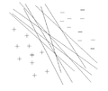
  Infinitely many Perceptron solutions

• 

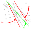
  Out of many how do we choose?

So with Perceptron, there can be infinitely many solutions you can get, where the training error will be zero. But the question is that among all these possible solution which one is the best. Intuitively we choose the solution with the largest margin between both classes. So if we choose the hyper-plane with the maximum margin between the two classes that could be a better solution. This makes sense because at test time, more points will be observed and they may be closer to the other class, so the safest choice for the hyper-plane would be the one farthest from both classes.

One of the great things about SVM is that not only it has solid theoretical guarantees, but also it works very well in practice.

To summarize:

What we mean by margin is the distance between the hyperplane and the closest point in a class.

If the data is Linearly separable, then there exists infinitely many solution hyperplanes. Of those, infinitely many hyperplanes one of them is the best choice for the solution. Then the best decision to make is the hyperplane which is furthest from both classes. So our goal is to find a hyperplane amoung all possible hyperplanes which is furthest from both classes. which is to find a Hyperplane that has maximum margin.

What we mean by margin is the distance between the hyperplane and the closest point in a class.

If the mean value were to be used instead of the closest point, then an outlier may pull the hyperplane into the data which would incorrectly classify the known data points. This is the reason why we use the closest point instead of the expected value.

Setting

What is $d_i$

• We assume that the data is linearly separable
• Our classifier will be of the form ${\mathit{\beta }}^T\mathbf{x}+{\beta }_0$
• We will assume that our labels are $y_i\in \{-1,1\}$

The goal is to classify the point ${\mathbf{x}}_{\mathbf{i}}$ based on the $sign\{d_i\}$ where $d_i$ is the signed distance between ${\mathbf{x}}_{\mathbf{i}}$ and the hyperplane.

Now we are going to check how far this point is from the hyperplane, and the parts on one side of the hyperplane will have a negative value and the parts on the other side will have a positive value. Points are classified by the sign of the data point. So ${\mathbf{x}}_{\mathbf{i}}$ would be classified using $d_i$

Side Note: A memory from the past of Dr. Ali Ghodsi

When the aforementioned Professor was a small child, grade 2. He was often careless with the accuracy of certain curly brackets, when writing what one can only assume was math proofs. One day, his teacher grew impatient and demanded that a page of perfect curly brackets be produced by the young Dr. (He may or may not have been a doctor at the time) And now, whenever Dr. Ghodsi writes a tidy curly bracket, he is reminded of this and it always brings a smile to his face.

From memories of the past.

(the number 20 was involved in the story, either the number of pages or the number of lines)

Case 1: Linearly Separable (Hard Margin)

In this case, the classifier will be ${\mathit{\beta }}^{\mathit{T}}+{\beta }_0$ and $y\in \{-1,1\}$ The classify point ${\mathit{x}}_{\mathit{i}}$ based on sign $\{d_i\}$, where $d_i$ is the digned distance between ${\mathit{x}}_{\mathit{i}}$ and the hyperplain.

Objective Function

Look at it being perpendicular

Observation 1: $\mathit{\beta }$ is orthogonal to hyper-plane. Because, for any two arbitrary points ${\mathbf{x}}_{\mathbf{1}}\mathbf{,}{\mathbf{x}}_{\mathbf{2}}$ on the plane we have:

${\mathit{\beta }}^T{\mathbf{x}}_{\mathbf{1}}+{\beta }_0=0$

${\mathit{\beta }}^T{\mathbf{x}}_{\mathbf{2}}+{\beta }_0=0$

So ${\mathit{\beta }}^T({\mathit{x}}_{\mathbf{1}}-{\mathit{x}}_{\mathbf{2}})=0$. Thus, ${\mathit{\beta }}^T\perp ({\mathit{x}}_{\mathbf{1}}-{\mathit{x}}_{\mathbf{2}})$, which implies that $\mathit{\beta }$ is a normal vector to the hyper-plane.

Observation 2: If ${\mathit{x}}_0$ is a point on the hyper-plane, then there exists a ${\beta }_0$ such that, ${\mathit{\beta }}^T{\mathit{x}}_{\mathbf{0}}+{\beta }_0=0$. So ${\mathit{\beta }}^T{\mathit{x}}_{\mathbf{0}}=-{\beta }_0$. This along with observation 1 imply there exists a ${\beta }_0$ such that, ${\mathit{\beta }}^T\mathit{x}=-{\beta }_0$ for all $\mathit{x}$ on the hyperplane.

Observation 3: Let $d_i$ be the signed distance of point ${\mathit{x}}_{\mathit{i}}$ from the plane. The $d_i$ is the projection of $({\mathit{x}}_{\mathit{i}}-{\mathit{x}}_{\mathbf{0}})$ on the direction of $\mathit{\beta }$. In other words, $d_i\propto {\mathit{\beta }}^T(\mathbf{x}\mathbf{-}{\mathbf{x}}_{\mathbf{0}})$.(normalize $\beta$)

$\begin{array}{rl}{d}_i& =\frac{{\mathit{\beta }}^T({\mathit{x}}_{\mathit{i}}-{\mathit{x}}_{\mathbf{0}})}{|\mathit{\beta }|}\\ & =\frac{{\mathit{\beta }}^{\mathit{T}}{\mathit{x}}_{\mathit{i}}-{\mathit{\beta }}^{\mathit{T}}{\mathit{x}}_{\mathbf{0}}}{|\mathit{\beta }|}\\ & =\frac{{\mathit{\beta }}^{\mathit{T}}{\mathit{x}}_{\mathit{i}}+{\beta }_0}{|\mathit{\beta }|}\end{array}$

Observation 4: Let margin be the distance between the hyper-plane and the closest point. Since $d_i$ is the signed distance between the hyperplane and point ${\mathit{x}}_{\mathit{i}}$, we can define the positive distance of point ${\mathit{x}}_{\mathit{i}}$ from the hyper-plane as $(y_i{d}_i)$.

$\begin{array}{rl}\text{Margin}& =min\{y_i{d}_i\}\\ & =min\{\frac{y_i({\mathit{\beta }}^T{\mathbf{x}}_{\mathbf{i}}+{\beta }_0)}{|\mathit{\beta }|}\}\end{array}$

Our goal is to maximize the margin. This is also known as the Max/Min problem in Optimization. When defining the hyperplane, what is important is the direction of $\mathit{\beta }$. Value of ${\beta }_0$ does not change the direction of the hyper-plane, it is only the distance from the origin. Note that if we assume that the points do not lie on the hyper-plane, then the margin is positive:

$\begin{array}{rlrl}{\displaystyle }& y_i({\mathit{\beta }}^T{\mathbf{x}}_{\mathbf{i}}+{\beta }_0)\ge 0& & \\ & y_i({\mathit{\beta }}^T{\mathbf{x}}_{\mathbf{i}}+{\beta }_0)\ge C& & \text{ for some positive C }\\ & y_i(\frac{{\mathit{\beta }}^T}{C}{\mathbf{x}}_{\mathbf{i}}+\frac{{\beta }_0}{C})\ge 1& & \text{ Divide by C}\\ & y_i({\mathit{\beta }}^{\ast T}{\mathbf{x}}_{\mathbf{i}}+{\beta }_0^{\ast })\ge 1& & \text{ By setting }{\mathit{\beta }}^{\ast }=\frac{\mathit{\beta }}{C},{\mathit{\beta }}_0^{\ast }=\frac{{\mathit{\beta }}_0}{C}\\ & y_i({\mathit{\beta }}^T{\mathbf{x}}_{\mathbf{i}}+{\beta }_0)\ge 1& & \text{ By setting }\mathit{\beta }\leftarrow {\mathit{\beta }}^{\ast },{\mathit{\beta }}_0\leftarrow {\mathit{\beta }}_0^{\ast }\end{array}$

So with a bit of abuse of notation we can assume that

$y_i({\mathit{\beta }}^T{\mathbf{x}}_{\mathbf{i}}+{\beta }_0)\ge 1$

Therefore, the problem translates to:

$min\{\frac{1}{|\mathit{\beta }|}\}$

So, it is possible to re-interpret the problem as:

$max\frac{1}{2}|\mathit{\beta }{|}^2$ s.t. $y_i({\mathit{\beta }}^T{\mathit{x}}_{\mathit{i}}+{\beta }_0)\ge 1$

$|\mathit{\beta }|$ could be any norm, but for simplicity we use L2 norm. We use $\frac{1}{2}|\mathit{\beta }{|}^2$ instead of $|\mathit{\beta }|$ to make the function differentiable. To solve the above optimization problem we can use Lagrange multipliers as follows

Support Vectors

Support vectors are the training points that determine the optimal separating hyperplane that we seek. Also, they are the most difficult points to classify and at the same time the most informative for classification.

Writing Lagrangian Form of Support Vector Machine

The Lagrangian form using Lagrange multipliers and constraints that are discussed below is introduced to ensure that the optimization conditions are satisfied, as well as finding an optimal solution (the optimal saddle point of the Lagrangian for the classic quadratic optimization). The problem will be solved in dual space by introducing ${\alpha }_i$ as dual constraints, this is in contrast to solving the problem in primal space as function of the betas. A simple algorithm for iteratively solving the Lagrangian has been found to run well on very large data sets, making SVM more usable. Note that this algorithm is intended to solve Support Vector Machines with some tolerance for errors - not all points are necessarily classified correctly. Several papers by Mangasarian explore different algorithms for solving SVM.

Dual form of the optimization problem:

$\begin{array}{rl}L(\mathit{\beta },{\beta }_0,\mathit{\alpha })& =\frac{1}{2}|\mathit{\beta }{|}^2-\sum _{i=1}^n{\alpha }_i[y_i({\mathit{\beta }}^{\mathit{T}}{\mathit{x}}_{\mathit{i}}+{\beta }_0)-1]\\ & =\frac{1}{2}|\mathit{\beta }{|}^2-{\mathit{\beta }}^T\sum _{i=1}^n{\alpha }_i{y}_i{\mathit{x}}_{\mathit{i}}-\sum _{i=1}^n{\alpha }_i{y}_i{\beta }_0-\sum _{i=1}^n{\alpha }_i\end{array}$

To find the optimal value, we set the derivatives equal to zero: $\frac{\partial L}{\partial \mathit{\beta }}=0$ and $\frac{\partial L}{\partial {\beta }_0}=0$.

$\begin{array}{rlrl}{\displaystyle }& \frac{\partial L}{\partial \mathit{\beta }}=\mathit{\beta }-\sum _{i=1}^n{\alpha }_i{y}_i{\mathit{x}}_{\mathit{i}}=0& ⟹& \mathit{\beta }=\sum _{i=1}^n{\alpha }_i{y}_i{\mathit{x}}_{\mathit{i}}\\ & \frac{\partial L}{\partial {\beta }_0}=-\sum _{i=1}^n{\alpha }_i{y}_i=0& ⟹& \sum _{i=1}^n{\alpha }_i{y}_i=0\end{array}$

To get the dual form of the optimization problem we replace the above two equations in definition of $L(\mathit{\beta },{\beta }_0,\mathit{\alpha })$. We get: $\begin{array}{rl}L(\mathit{\beta },{\beta }_0,\mathit{\alpha })& =\frac{1}{2}{\mathit{\beta }}^T\mathit{\beta }-{\mathit{\beta }}^T\sum _{i=1}^n{\alpha }_i{y}_i{\mathit{x}}_{\mathit{i}}-\sum _{i=1}^n{\alpha }_i{y}_i{\beta }_0-\sum _{i=1}^n{\alpha }_i\\ & =\frac{1}{2}{\mathit{\beta }}^T\sum _{i=1}^n{\alpha }_i{y}_i{\mathit{x}}_{\mathit{i}}-{\mathit{\beta }}^T\sum _{i=1}^n{\alpha }_i{y}_i{\mathit{x}}_{\mathit{i}}-0+\sum _{i=1}^n{\alpha }_i\\ & =-\frac{1}{2}{\mathit{\beta }}^T\sum _{i=1}^n{\alpha }_i{y}_i{\mathit{x}}_{\mathit{i}}+\sum _{i=1}^n{\alpha }_i\\ & =-\frac{1}{2}\sum _{i=1}^n{\alpha }_i{y}_i{\mathit{x}}_{\mathit{i}}^T\sum _{i=1}^n{\alpha }_i{y}_i{\mathit{x}}_{\mathit{i}}+\sum _{i=1}^n{\alpha }_i\\ & =\sum _{i=1}^n{\alpha }_i-\frac{1}{2}\sum _{i=1}^n\sum _{j=1}^n{\alpha }_i{\alpha }_j{y}_i{y}_j{\mathit{x}}_{\mathit{i}}^T{\mathit{x}}_{\mathit{j}}\end{array}$

The above function is a dual objective function, so we should minimize it:

$\begin{array}{rl}\underset{\alpha }{min}& \sum _{i=1}^n{\alpha }_i-\frac{1}{2}\sum _{i=1}^n\sum _{j=1}^n{\alpha }_i{\alpha }_j{y}_i{y}_j{\mathit{x}}_{\mathit{i}}^T{\mathit{x}}_{\mathit{j}}\\ s.t.& {\alpha }_i\ge 0\\ & \sum _{i=1}^n{\alpha }_i{y}_i=0\end{array}$

The dual function is a quadratic function of several variables subject to linear constraints. This optimization problem is called Quadratic Programming and is much easier than the primal function. It is possible to to write to dual form using matrices:

$\begin{array}{rl}\underset{\alpha }{min}& {\mathit{\alpha }}^T\mathbf{1}-\frac{1}{2}{\mathit{\alpha }}^{T}S\mathit{\alpha }\\ s.t.& \mathit{\alpha }\ge 0\\ & {\mathit{\alpha }}^{T}y=0\\ & S=([y_1,\dots ,y_n]\odot X{)}^T([y_1,\dots ,y_n]\odot X)\end{array}$

Since $S=([y_1,\dots ,y_n]\odot X{)}^T([y_1,\dots ,y_n]\odot X)$, S is a positive semi-definite matrix. This means that the dual function is convex.[5]. This means that the dual function does not have any local minimum that is not global. So it is relatively easy to find the global minimum.

Discussion on the Dual of the Lagrangian

As mentioned in the previous section, solving the dual form of the Lagrangian requires quadratic programming. Quadratic programming can be used to minimize a quadratic function subject to a set of constraints. In general, for a problem with N variables, the quadratic programming solution has a computational complexity of $O(N^3)$ <ref name="CMBishop" />. The original problem formulation only has (d+1) variables that need to be found (i.e. the values of $\beta$ and ${\beta }_0$), where d is the dimensionality of the data points. However, the dual form of the Lagrangian has n variables that need to be found (i.e. all the $\alpha$ values), where n is the number of data points. It is likely that n is larger than (d+1) (i.e. the number of data points is larger than the dimensionality of the data plus 1), which makes the dual form of the Lagrangian seem computationally inefficient <ref name="CMBishop" />. However, the dual of the Lagrangian allows the inner product $x_i^T{x}_j$ to be expressed using a kernel formulation which allows the data to be transformed into higher feature spaces and thus allowing seemingly non-linearly separable data points to be separated, which is a highly useful feature described in more detail in the next class <ref name="CMBishop" />.

Support Vector Machine Continued (Lecture: Nov.1, 2011)

Previous lecture we considered the case when data is linearly separable. The goal of the Support Vector Machine classifier is to find the hyper-plane that maximizes the margin from each of the two classes. We derived the following optimization problem based on the SVM methodology:

$\underset{\beta ,{\beta }_0}{min}\frac{1}{2}{|\mathit{\beta }|}^2$

Subject to the constraint:

$y_i({\mathit{\beta }}^T{\mathbf{x}}_i+{\beta }_0)\ge 1$

This is the primal form of the optimization problem. Then we derived the dual of this problem:

$\underset{\alpha }{max}\sum _i{\alpha }_i-\frac{1}{2}\sum _i\sum _j{\alpha }_i{\alpha }_j{y}_i{y}_j{\mathbf{x}}_i^T{\mathbf{x}}_j$

Subject to constraints:

${\alpha }_i\ge 0$

$\sum _i{\alpha }_i{y}_i=0$

The is quadratic programming problem. QP problems have been thoroughly studied and that can be efficiently solved. This particular problem has a convex objective function as well as convex constraints. This makes solving the problem easier and ensures the computed solution is the global maximum. These properties are of significant important for classifiers and thus are one of the most important strengths of the SVM classifier.

We are able to find $\beta$ when $\alpha$ is found:

$\mathit{\beta }=\sum _i{\alpha }_i{y}_i{\mathbf{x}}_i$

But in order to find the hyper-plane uniquely we need also to find ${\beta }_0$.

When finding the dual objective function, there are set of conditions called KKT that should be satisfied.

KKT Conditions

KKT stands for Karush-Kuhn-Tucker (initially named after Kuhn and Tucker's work in the 1950's, however, it was later discovered that Karush had stated the conditions back in the late 1930's) <ref name="CMBishop" />

Suppose we want to find $mi{n}_{x}f(x)$ subject to the constraint $g_i(x)\ge 0,\mathrm{\forall }x$ :

$\mathcal{L}(x,{\alpha }_i)=f(x)-\sum _i{\alpha }_i{g}_i(x)$

If $x^{\ast }$ is the optimal point , the necessary conditions for $x^{\ast }$ to be the local minimum :

1) $\frac{\partial \mathcal{L}}{\partial x}(x^{\ast })=0$ that is $f^{\prime }(x^{\ast })-{\mathrm{\Sigma }}_i{\alpha }_i{g}^{\prime }(x^{\ast })=0$

2) ${\alpha }_i\ge 0,$ dual feasibility

3) ${\alpha }_i{g}_i(x^{\ast })=0,$ complementary slackness

4) $g_i(x^{\ast })\ge 0,$ primal feasibility

If any of the above four conditions are not satisfied, then the primal function is not feasible.

Looking more closely at condition 3:

${\alpha }_i{g}_i(x^{\ast })=0$

${\alpha }_i[y_i({\beta }^T{x}_i+{\beta }_0)-1]=0$

We see that this is at the optimal point.

It is obvious that we can have either ${\alpha }_i\ge 0$ or $y_i({\beta }^T{x}_i+{\beta }_0)\ge 1$.

If ${\alpha }_i>0$, this gives $y_i({\beta }^T{x}_i+{\beta }_0)=1$; then the point $x_i$ is on the margin of the hyper-plane and this point is called a support vector.

If $y_i({\beta }^T{x}_i+{\beta }_0)\ge 1$, we have ${\alpha }_i=0$, in this case, the point $x_i$ is away from the margin of the hyper-plane.

Note here that ${\alpha }_i$ is positive if and only if $x_i$ is on the margin. Thus $x_i$ that correspond to positive ${\alpha }_i$ are called support vectors. For all other points not on the margin ${\alpha }_i$ is 0. This essentially means that only the support vectors will affect the hyperplane found using SVM, thus SVM is a relatively robust classifier (i.e. it is not affected by outlying points).

To compute ${\beta }_0$, we need to choose any ${\alpha }_i>0$, this will satisfy:

$y_i({\beta }^T{x}_i+{\beta }_0)=1$.

We can compute $\beta =\sum _i{\alpha }_i{y}_i{x}_i$, substitute $\beta$ in $y_i({\beta }^T{x}_i+{\beta }_0)=1$ and solve for ${\beta }_0$.

$\left[\begin{array}{c}x\\ y\end{array}\right]\to \left[\begin{array}{c}{x}^2\\ y^2\\ \sqrt{2}xy\end{array}\right]$

$k(x,y)={\varphi }^T(x)\varphi (y)$

$\left[\begin{array}{c}{x}_1\\ y_1\end{array}\right]\to \left[\begin{array}{c}{x}_1^2\\ y_1^2\\ \sqrt{2}{x}_1{y}_1\end{array}\right]$

$\left[\begin{array}{c}{x}_2\\ y_2\end{array}\right]\to \left[\begin{array}{c}{x}_2^2\\ y_2^2\\ \sqrt{2}{x}_2{y}_2\end{array}\right]$

${\left[\begin{array}{c}{x}_1^2\\ y_1^2\\ \sqrt{2}{x}_1{y}_1\end{array}\right]}^T\ast \left[\begin{array}{c}{x}_2^2\\ y_2^2\\ \sqrt{2}{x}_2{y}_2\end{array}\right]=K(\left[\begin{array}{c}{x}_1\\ y_1\end{array}\right],\left[\begin{array}{c}{x}_2\\ y_2\end{array}\right])$

$\sum _i{\alpha }_i-\frac{1}{2}\sum _{ij}{\alpha }_i{\alpha }_j{y}_i{y}_j{\mathbf{x}}_i^T{\mathbf{x}}_j$

where ${\mathbf{x}}_i^T{\mathbf{x}}_j={\varphi }^T(x)\varphi (y)=k(x_i,x_j)$

$\left[\begin{array}{cccc}k(x_1,x_1)& k(x_1,x_2)& \cdots & k(x_1,x_n)\\ ⋮& ⋮& ⋮& ⋮\\ k(x_n,x_1)& k(x_n,x_2)& \cdots & k(x_n,x_n)\end{array}\right]$

Whatever we derived so far was based on the assumption that the data is linearly separable but that might not be the case always and it might be impossible to find a hyper-plane that completely separates two class of data . This case is called hard margin hyper-plane.

Kernel Trick

In most of the real world cases the data points are not linearly separable. How can the above methods be generalized to the case where the decision function is not a linear function of the data? Boser, Guyon and Vapnik, 1992, showed that a rather old trick (Aizerman, 1964) can be used to accomplish this in an astonishingly straightforward way. First notice that the only way in which the data appears in the dual-form optimization problem is in the form of dot products: ${\mathbf{x}}_i^T.{\mathbf{x}}_j$ . Now suppose we first use a non-linear operator $\mathrm{\Phi }\mathbf{(}x)$ to map the data points to some other higher dimensional space (possibly infinite dimensional) $\mathcal{H}$ (called Hilbert space or feature space), where they can be classified linearly. Figure below illustrates this concept:

File:kernell trick.jpg

Mapping of not-linearly separable data points in a two-dimensional space to a three-dimensional space where they can be linearly separable by means of a kernel function.

In other words, a linear learning machine can be employed in the higher dimensional feature space to solve the original non-linear problem. Then of course the training algorithm would only depend on the data through dot products in $\mathcal{H}$, i.e. on functions of the form $<{\mathrm{\Phi }}^T({\mathbf{x}}_i).\mathrm{\Phi }({\mathbf{x}}_j)>$. Note that the actual mapping $\mathrm{\Phi }\mathbf{(}x)$ does not need to be known, only the inner product of the mapping is needed for modifying the support vector machine such that it can separate non-linearly separable data. Avoiding the actual mapping to the higher dimensional space is preferable, because higher dimensional spaces may have problems due to the curse of dimensionality.

So the hypothesis in this case would be

$f(\mathbf{x})={\mathit{\beta }}^T\mathrm{\Phi }(\mathbf{x})+{\beta }_0$

which is linear in terms of the new space that $\mathrm{\Phi }(\mathbf{x})$ maps the data to, but non-linear in the original space. Now we can extend all the presented optimization problems for the linear case, for the transformed data in the feature space. If we define the kernel function as

$K({\mathbf{x}}_i,{\mathbf{x}}_j)=<\mathrm{\Phi }({\mathbf{x}}_i),\mathrm{\Phi }({\mathbf{x}}_j)>$

where $\mathrm{\Phi }$ is a mapping from input space to an (inner product) feature space. Then the corresponding dual form is

$L(\mathit{\alpha })=\sum _{i=1}^n{\alpha }_i-\frac{1}{2}\sum _{i=1}^n\sum _{j=1}^n{\alpha }_i{\alpha }_j{y}_i{y}_{j}K({\mathbf{x}}_i,{\mathbf{x}}_j)$

subject to $\sum _{i=1}^n{\alpha }_i{y}_i=0{\alpha }_i\ge 0,i=1,\cdots ,n$

The cost function $L(\mathit{\alpha })$ is convex and quadratic in terms of the unknown parameters. This problem is solved through quadratic programming. The KKT conditions for this equation lead to the following final decision rule:

$L(\mathbf{x},{\mathit{\alpha }}^{\ast },{\beta }_0)=\sum _{i=1}^{N_{sv}}{y}_i{\alpha }_i^{\ast }K({\mathbf{x}}_i,\mathbf{x})+{\beta }_0$

where $N_{sv}$ and ${\alpha }_i$ denote number of support vectors and the non-zero Lagrange multipliers corresponding to the support vectors respectively.

Several typical choices of kernels are linear, polynomial, Multi-Layer Perceptron (MLP) and Gaussian or Radial Basis Function (RBF) kernel. Their expressions are as following:

Linear kernel: $K({\mathbf{x}}_i,{\mathbf{x}}_j)={\mathbf{x}}_i^T{\mathbf{x}}_j$

Polynomial kernel: $K({\mathbf{x}}_i,{\mathbf{x}}_j)=(1+{\mathbf{x}}_i^T{\mathbf{x}}_j{)}^p$

MLP kernel: $K({\mathbf{x}}_i,{\mathbf{x}}_j)=\tanh (k_1{\mathbf{x}}_i^T{\mathbf{x}}_j+k_2)$

Gaussian (RBF) kernel: $K({\mathbf{x}}_i,{\mathbf{x}}_j)=\exp (\frac{-[({\mathbf{x}}_i-{\mathbf{x}}_j){]}^2}{2{\sigma }^2})$

Radial Basis: $K({\underset{―}{x}}_i,{\underset{―}{x}}_j)=exp(-\gamma \Vert {\underset{―}{x}}_i-{\underset{―}{x}}_j{\Vert }^2),\gamma >0$

Sigmoid: $K({\underset{―}{x}}_i,{\underset{―}{x}}_j)=tanh(\gamma {\underset{―}{x}}_i^T{\underset{―}{x}}_j+r)$.

where, $\gamma$, $r$, and $d$ are all kernel parameters.

Kernel functions satisfying Mercer's conditions not only enables implicit mapping of data from input space to feature space but also ensure the convexity of the cost function which leads to the unique optimum. Mercer condition states that a continuous symmetric function $K\mathbf{(}x,y)$ must be positive semi-definite to be a kernel function which can be written as inner product between the data pairs. Note that we would only need to use K in the training algorithm, and would never need to explicitly even know what $\mathrm{\Phi }$ is.

In the case of Gaussian or RBF kernel for example, $\mathcal{H}$ is infinite dimensional, so it would not be very easy to work with $\mathrm{\Phi }$ explicitly. However, if one replaces $<({\mathbf{x}}_i).({\mathbf{x}}_j)>$ by $K({\mathbf{x}}_i,{\mathbf{x}}_j)$ everywhere in the training algorithm, the algorithm will happily produce a support vector machine which lives in an infinite dimensional space, and furthermore do so in roughly the same amount of time it would take to train on the un-mapped data. All the considerations of the previous sections hold, since we are still doing a linear separation, but in a different space.

The choice of which kernel would be best for a particular application has to be determined through trial and error. Normally, the Gaussian or RBF kernel are best suited for classification tasks including SVM.

The video below shows a graphical illustration of how a polynomial kernel works to a get better sense of kernel concept:

Mapping data points to a higher dimensional space using a polynomial kernel

Kernel Properties

Kernel functions must be continuous, symmetric, and most preferably should have a positive (semi-) definite Gram matrix. Kernels which are said to satisfy the Mercer's theorem are positive semi-definite, meaning their kernel matrices have no non-negative Eigen values. The use of a positive definite kernel insures that the optimization problem will be convex and solution will be unique. <ref> Reference:http://crsouza.blogspot.com/2010/03/kernel-functions-for-machine-learning.html#kernel_properties </ref>

Case 2: Linearly Non-Separable Data (Soft Margin)

The original SVM was specifically made for separable data. But, this is a very strong requirement, so it was suggested by Vladimir Vapnik and Corinna Cortes later on to remove this requirement. This is called Soft Margin Support Vector Machine. One of the advantages of SVM is that it is relatively easy to generalize it to the case that the data is not linearly separable.

In the case when 2 data sets are not linearly separable, it is impossible to have a hyperplane that completely separates 2 classes of data. In this case the idea is to minimize the number of points that cross the margin and are miss-classified .So we are going to minimize that are going to violate the constraint:

$y_i({\beta }^T{x}_i+{\beta }_0)\ge 1$

Hence we allow some of the points to cross the margin (or equivalently violate our constraint) but on the other hand we penalize our objective function (so that the violations of the original constraint remains low):

$min(1/2|\beta {|}^2+\gamma \sum _i{\zeta }_i)$

And now our constraint is as follows:

$y_i({\beta }^T{x}_i+{\beta }_0)\ge 1-{\zeta }_i$

${\zeta }_i\ge 0$

We have to check that all KKT conditions are satisfied:

$\mathcal{L}(\beta ,{\beta }_0,{\zeta }_i,{\alpha }_i,{\lambda }_i)=1/2|\beta {|}^2+\gamma \sum _i{\zeta }_i-\sum _i{\alpha }_i(y_i({\beta }^T{x}_i+{\beta }_0)-1+{\zeta }_i)-\sum _i{\lambda }_i{\zeta }_i$

$1)\frac{\partial \mathcal{L}}{\partial \beta }=\beta -\sum _i{\alpha }_i{y}_i{x}_i\Rightarrow \beta =\sum _i{\alpha }_i{y}_i{x}_i$

$2)\frac{\partial \mathcal{L}}{\partial {\beta }_0}=\sum _i{\alpha }_i{y}_i=0$

$3)\frac{\partial \mathcal{L}}{\partial {\zeta }_i}=\gamma -{\alpha }_i-{\lambda }_i$

Now we have to write this into a Lagrangian form.

Support Vector Machine Continued (Lecture: Nov. 3, 2011)

Case 2: Linearly Non-Separable Data (Soft Margin [6]) Continued

Recall from last time that soft margins are used instead of hard margins when we are using SVM to classify data points that are not linearly separable.

Soft Margin SVM derivation of dual

The soft-margin SVM optimization problem is defined as:

$min(\frac{1}{2}|\mathit{\beta }{|}^2+\gamma \sum _i{\zeta }_i)$ subject to the constraints $y_i({\mathit{\beta }}^T{\mathit{x}}_{\mathit{i}}+{\beta }_0)\ge 1-{\zeta }_i$, here we have ${\zeta }_i\ge 0$.

In other words, we have relaxed the constraint for each ${\mathit{x}}_{\mathit{i}}$ so that it can violate the margin by an amount ${\zeta }_i$. As such, we want to make sure that all ${\zeta }_i$ values are as small as possible. So, we penalize them in the objective function by a factor of some chosen $\gamma$.

Now we can define our Lagrangian:

$L(\mathit{\beta },{\beta }_0,{\zeta }_i,{\alpha }_i,{\lambda }_i)=\frac{1}{2}|\mathit{\beta }{|}^2+\gamma \sum _i{\zeta }_i-\sum _i{\alpha }_i[y_i({\mathit{\beta }}^T{\mathit{x}}_{\mathit{i}}+{\beta }_0)-1+{\zeta }_i]-\sum _i{\lambda }_i{\zeta }_i$

Our K.K.T. conditions are as follows:

$\begin{array}{rl}1)& \frac{\partial \mathcal{L}}{\partial \mathit{\beta }}=\mathit{\beta }-\sum _i{\alpha }_i{y}_i{\mathit{x}}_{\mathit{i}}=0\\ & ⟹\mathit{\beta }=\sum _i{\alpha }_i{y}_i{\mathit{x}}_{\mathit{i}}\\ & \frac{\partial \mathcal{L}}{\partial {\beta }_0}=\sum _i{\alpha }_i{y}_i=0\\ & \frac{\partial \mathcal{L}}{\partial {\zeta }_i}=\gamma -{\alpha }_i-{\lambda }_i=0\\ 2)& {\alpha }_i\ge 0,{\lambda }_i\ge 0\\ 3)& {\alpha }_i[y_i({\mathit{\beta }}^T{\mathit{x}}_{\mathit{i}}+{\beta }_0)-1+{\zeta }_i]=0,{\lambda }_i{\zeta }_i=0\\ 4)& y_i({\mathit{\beta }}^T{\mathit{x}}_{\mathit{i}}+{\beta }_0)\ge 1-{\zeta }_i\end{array}$

So, simplifying the Lagrangian the same way we did with the hard margin case, we get the following:

$\begin{array}{rl}L& =\frac{1}{2}\sum _{i,j}{\alpha }_i{\alpha }_j{y}_i{y}_j{\mathit{x}}_{\mathit{i}}^T{\mathit{x}}_{\mathit{j}}+\gamma \sum _i{\zeta }_i-\sum _{i,j}{\alpha }_i{\alpha }_j{y}_i{y}_j{\mathit{x}}_{\mathit{i}}^T{\mathit{x}}_{\mathit{j}}-{\beta }_0\sum _i{\alpha }_i{y}_i+\sum _i{\alpha }_i-\sum _i{\alpha }_i{\zeta }_i-\sum _i{\lambda }_i{\zeta }_i\\ & =-\frac{1}{2}\sum _{i,j}{\alpha }_i{\alpha }_j{y}_i{y}_j{\mathit{x}}_{\mathit{i}}^T{\mathit{x}}_{\mathit{j}}+\sum _i{\alpha }_i-0+(\sum _i\gamma {\zeta }_i-\sum _i{\alpha }_i{\zeta }_i-\sum _i{\lambda }_i{\zeta }_i)\\ & =-\frac{1}{2}\sum _{i,j}{\alpha }_i{\alpha }_j{y}_i{y}_j{\mathit{x}}_{\mathit{i}}^T{\mathit{x}}_{\mathit{j}}+\sum _i{\alpha }_i+\sum _i(\gamma -{\alpha }_i-{\lambda }_i){\zeta }_i\\ & =-\frac{1}{2}\sum _{i,j}{\alpha }_i{\alpha }_j{y}_i{y}_j{\mathit{x}}_{\mathit{i}}^T{\mathit{x}}_{\mathit{j}}+\sum _i{\alpha }_i\end{array}$

subject to ${\alpha }_i\ge 0,\sum _i{\alpha }_i{y}_i=0,{\lambda }_i\ge 0$. Notice that the Lagrangian is the exact same as the hard margin case. The only difference with the soft margin case is the additional constraint ${\lambda }_i\ge 0$. However, $\gamma$ doesn't actually appear directly in the objective function. But, we can discern the following:

${\gamma }_i=0⟹{\alpha }_i=\gamma$

${\gamma }_i>0⟹{\alpha }_i<\gamma$

Thus, we can derive that the only difference with the soft margin case is the constraint $0\le {\alpha }_i\le \gamma$. This problem can be solved with quadratic programming.

Soft Margin SVM formulation summary

In summary, the primal form of the soft-margin SVM is given by:

$\begin{array}{rl}\underset{\mathit{\beta },\mathit{\zeta }}{min}& \frac{1}{2}|\mathit{\beta }{|}^2+\gamma \sum _i{\zeta }_i\\ \text{s.t. }& y_i({\mathit{\beta }}^T{\mathit{x}}_{\mathit{i}}+{\beta }_0)\ge 1-{\zeta }_i,i=1,...,M\end{array}$

The corresponding dual form which we derived above is:

$\begin{array}{rl}\underset{\mathit{\alpha }}{max}& \sum _i{\alpha }_i-\frac{1}{2}\sum _{i,j}{\alpha }_i{\alpha }_j{y}_i{y}_j{\mathit{x}}_{\mathit{i}}^T{\mathit{x}}_{\mathit{j}}\\ \text{s.t. }& \sum _i{\alpha }_i{y}_i=0\\ & 0\le {\alpha }_i\le \gamma ,i=1,...,M\end{array}$

Note, the soft-margin dual objective is identical to hard margin dual objective! The only difference is now ${\alpha }_i$ variables cannot be unbounded and are restricted to be a maximum of $\gamma$. This restriction allows the optimization problem to become feasible when the data is non-seperable. In the hard-margin case, when ${\alpha }_i$ is unbounded there may be no finite maximum for the objective and we would not be able to converge to a solution.

Also note, $\gamma$ is a model parameter and must be chosen to a fixed constant. It controls the size of margin versus violations. In a data set with a lot of noise (or non-seperability) you may want to choose a smaller $\gamma$ to ensure a large margin. In practice, $\gamma$ is chosen by cross-validation---which tests the model on a held out sample to determine which $\gamma$ gives the best result. However, it may be troublesome to work with $\gamma$ since $\gamma \in (0,\mathrm{\infty })$. So often a variant formulation, known as $\nu$-SVM is used which uses a better scaled parameter $\nu \in (0,1)$ instead of $\gamma$ to balance margin versus separability.

Finally note that as $\gamma \to \mathrm{\infty }$, the soft-margin SVM converges to hard-margin, as we do not allow any violation.

Soft Margin SVM problem interpretation

Like in the case of hard-margin the dual formulation for soft-margin given above allows us to interpret the role of certain points as support vectors.

We consider three cases:

Case 1: ${\alpha }_i=\gamma$

From KKT condition 1 (third part), $\gamma -{\alpha }_i-{\lambda }_i=0$ implies ${\lambda }_i=0$.

From KKT condition 3 (second part) ${\lambda }_i{\zeta }_i=0$ this now suggests ${\zeta }_i>0$.

Thus this is a point that violates the margin, and we say $x_i$ is inside the margin.

Case 2: ${\alpha }_i=0$

From KKT condition 1 (third part), $\gamma -{\alpha }_i-{\lambda }_i=0$ implies ${\lambda }_i>0$.

From KKT condition 3 (second part) ${\lambda }_i{\zeta }_i=0$ this now implies ${\zeta }_i=0$.

Finally, from KKT condition 3 (first part), $y_i({\mathit{\beta }}^T{\mathit{x}}_{\mathit{i}}+{\beta }_0)>1-{\zeta }_i$, and since ${\zeta }_i=0$, the point is classified correctly and we say $x_i$ is outside the margin. In particular, $x_i$ does not play a role in determining the classifier and if we ignored it, we would get the same result.

Case 3: $0<{\alpha }_i<\gamma$

From KKT condition 1 (third part), $\gamma -{\alpha }_i-{\lambda }_i=0$ implies ${\lambda }_i>0$.

From KKT condition 3 (second part) ${\lambda }_i{\zeta }_i=0$ this now implies ${\zeta }_i=0$.

Finally, from KKT condition 3 (first part), $y_i({\mathit{\beta }}^T{\mathit{x}}_{\mathit{i}}+{\beta }_0)=1-{\zeta }_i$, and since ${\zeta }_i=0$, the point is on the margin and we call it a support vector.

These three scenarios are depicted in Fig..

Soft Margin SVM with kernel

Like hard-margin SVM, we can use the kernel trick to find a non-linear classifier using the dual formulation.

In particular, we define a non-linear mapping for ${\mathit{x}}_{\mathit{i}}$ as $\mathrm{\Phi }({\mathit{x}}_{\mathit{i}})$, then in dual objective we compute ${\mathrm{\Phi }}^T({\mathit{x}}_{\mathit{i}})\mathrm{\Phi }({\mathit{x}}_{\mathit{j}})$ instead of ${\mathit{x}}_{\mathit{i}}^T{\mathit{x}}_{\mathit{j}}$. Using a kernel function $K({\mathit{x}}_{\mathit{i}},{\mathit{x}}_{\mathit{j}})={\mathrm{\Phi }}^T({\mathit{x}}_{\mathit{i}})\mathrm{\Phi }({\mathit{x}}_{\mathit{j}})$ from the list provided in the previous lecture notes, we then do not need to explicitly map $\mathrm{\Phi }({\mathit{x}}_{\mathit{i}})$.

The dual problem we solve is:

$\begin{array}{rl}\underset{\mathit{\alpha }}{max}& \sum _i{\alpha }_i-\frac{1}{2}\sum _{i,j}{\alpha }_i{\alpha }_j{y}_i{y}_{j}K({\mathit{x}}_{\mathit{i}},{\mathit{x}}_{\mathit{j}})\\ \text{s.t. }& \sum _i{\alpha }_i{y}_i=0\\ & 0\le {\alpha }_i\le \gamma ,i=1,...,M\end{array}$

where $K({\mathit{x}}_{\mathit{i}},{\mathit{x}}_{\mathit{i}})$ is an appropriate kernel function specification.

Soft Margin SVM implementation

The SVM optimization problem is a quadratic program and we can use any quadratic solver to accomplish this. For example, matlab's optimization toolbox provides quadprog. Alternatively, CVX (by Stephen Boyd) is an excellent optimization toolbox that integrates with matlab and allows one to enter convex optimization problems as though they are written on paper (and it is free).

We prefer to solve the dual since it is an easier problem (and also allows to use a Kernel). Using CVX this would be coded as

K = X*X';           % Linear kernel
H = (y*y') .* K;
cvx_begin 
    variable  alpha(M,1);
    maximize  (sum(alpha) - 0.5*alpha'*H*alpha)
    subject to
         y'*alpha == 0; 
         alpha >= 0;
         alpha <= gamma
cvx_end

which provides us with optimal $\mathit{\alpha }$.

Now we can obtain ${\beta }_0$ by using any point on the margin (i.e. $0<{\alpha }_i<\gamma$), and solving

$y_i(\sum _j{y}_j{\alpha }_{j}K({\mathit{x}}_{\mathit{j}},{\mathit{x}}_{\mathit{i}})+{\beta }_0)=1$

Note, $K({\mathit{x}}_{\mathit{i}},{\mathit{x}}_{\mathit{j}})={\mathit{x}}_{\mathit{i}}^T{\mathit{x}}_{\mathit{j}}$ can also be the linear kernel.

Finally, we can classify a new data point $\mathit{x}$, according to

$h(\mathit{x})=\{\begin{array}{l}+1,\text{if }\sum _j{y}_j{\alpha }_{j}K({\mathit{x}}_{\mathit{j}},\mathit{x})+{\beta }_0>0\\ -1,\text{if }\sum _j{y}_j{\alpha }_{j}K({\mathit{x}}_{\mathit{j}},\mathit{x})+{\beta }_0<0\end{array}$

Multiclass Support Vector Machines

A number of approaches exist for applying SVMs to classification tasks with more than two classes. The most straightforward approach given $k$ classes, is to use $k$ separate SVMs trained using the one-versus-the-rest approach, which basically trains the $i^{th}$ SVM such that the $i^{th}$ class is the "first class" (where $i=1,2,...k$) and the remaining $k-1$ classes are the "second class" for the $i^{th}$ SVM <ref name="CMBishop" />. Problems arise with this method as a point may be classified as different classes by each of the SVMs, because the class boundaries found by all SVMs may not be consistent such that each point belongs only to one class. Furthermore, the ratio of data points between the two classes in the one-versus-the-rest approach is not well balanced (the $k-1$ classes are likely to have a lot more points than the $i^{th}$ class) <ref name="CMBishop" />.

Variations of the one-versus-the-rest approach exist to address its problems:

• The class labels of each SVM can be changed from +1 and -1 to +1 (for the $i^{th}$ class) and $\frac{-1}{k-1}$ (for the remaining $k-1$ classes) in an attempt to counterbalance the unbalanced number of data points for each class <ref>Y. Lee, Y. Lin, and G. Wahba, "Multicategory Support Vector Machines," Technical Report, 2001</ref>.
• The $k$ SVMs can be trained at the same time using one objective function <ref>J. Weston and C. Watkins, "Multi-class Support Vector Machines," Proceedings ESANN, 1999</ref>.

Advantages of Support Vector Machines

• SVMs provide a good out-of-sample generalization. This means that, by choosing an appropriate generalization grade,

SVMs can be robust, even when the training sample has some bias. This is mainly due to selection of optimal hyperplane.

• SVMs deliver a unique solution, since the optimality problem is convex. This is an advantage compared

to Neural Networks, which have multiple solutions associated with local minima and for this reason may not be robust over different samples.

• State-of-the-art accuracy on many problems.
• SVM can handle any data types by changing the kernel.

Disadvantages of Support Vector Machines

• Difficulties in choice of the kernel (Which we will study about in future).

• limitation in speed and size, both in training and testing

• Discrete data presents another problem, although with suitable rescaling excellent results have nevertheless been obtained.

• The optimal design for multiclass SVM classifiers is a further area for research.

• A problem with SVMs is the high algorithmic complexity and extensive memory requirements of the required quadratic programming in large-scale tasks.

The Naive Bayes Classifier

The naive Bayes classifier is a very simple (and often effective) classifier based on Bayes rule. For further reading check [7]

Bayes assumption is that all the features are conditionally independent given the class label. Even though this is usually false (since features are usually dependent), the resulting model is easy to fit and works surprisingly well.

Each feature or variable $x_{ij}$ is independent for $j=1,...,d$, where ${\mathbf{x}}_i\in {\mathbb{R}}^d$.

Thus the Bayes classifier is $h(\mathbf{x})=\arg \underset{k}{max}{\pi }_k{f}_k(\mathbf{x})$

where ${\hat{f}}_k(\mathbf{x})={\hat{f}}_k(x_1{x}_2...x_d)=\prod _{j=1}^d{\hat{f}}_{kj}(x_j)$.

We can see this a direct application of Bayes rule $P(Y=k|X=\mathbf{x})=\frac{P(X=\mathbf{x}|Y=y)P(Y=y)}{P(X=\mathbf{x})}=\frac{f_k(\mathbf{x}){\pi }_k}{\sum _k{f}_k{\pi }_k}$,

with $f_k(\mathbf{x})=f(x^1)f(x^2)...f(x^d)$ and $\mathbf{x}\in {\mathbb{R}}^d$.

Note, earlier we assume class-conditional densitites which were multivariate normal with a dense covariance matrix. In this case we are forcing the covariance matrix to be a diagonal. This simplification, while not realistic, can provide a more robust model.

K-Nearest-Neighbors(k-NN)

Classifying x by assigning it the label most frequently represented among k nearest samples and use a voting scheme.

Given a data point x, find the k nearest data points to x and classify x using the majority vote of these k neighbors (k is a positive integer, typically small.) If k=1, then the object is simply assigned to the class of its nearest neighbor.

1. Ties can be broken randomly.
2. k can be chosen by cross-validation
3. k-nearest neighbor algorithm is sensitive to the local structure of the data<ref>

http://www.saylor.org/site/wp-content/uploads/2011/02/Wikipedia-k-Nearest-Neighbor-Algorithm.pdf</ref>.

1. Nearest neighbor rules in effect compute the decision boundary in an implicit manner.

Requirements of k-NN:

<ref>http://courses.cs.tamu.edu/rgutier/cs790_w02/l8.pdf</ref>

1. An integer k
2. A set of labeled examples (training data)
3. A metric to measure “closeness”

Advantages:

1. Able to obtain optimal solution in large sample.
2. Simple implementation
3. There are some noise reduction techniques that work only for k-NN to improve the efficiency and accuracy of the classifier.

Disadvantages:

1. If the training set is too large, it may have poor run-time performance.
2. k-NN is very sensitive to irrelevant features since all features contribute to the similarity and thus to classification.<ref>

http://www.google.ca/url?sa=t&rct=j&q=k%20nearest%20neighbors%20disadvantages&source=web&cd=1&ved=0CCIQFjAA&url=http%3A%2F%2Fciteseerx.ist.psu.edu%2Fviewdoc%2Fdownload%3Fdoi%3D10.1.1.100.1131%26rep%3Drep1%26type%3Dpdf&ei=3feyToHMG8Xj0QGOoMDKBA&usg=AFQjCNFF1XsYgZy1W2YLQMNTq_7s07mfqg&sig2=qflY4MffEHwP9n-WpnWMdg</ref>

1. small training data can lead to high misclassification rate.

Extensions and Applications

In order to improve the obtained results, we can do following:

1. Preprocessing: smoothing the training data (remove any outliers and isolated points)
2. Adapt metric to data

Besides classification, k-nearest-neighbours is useful for other tasks as well. For example, the k-NN has been used in Regression or Product Recommendation system<ref> http://www.cs.ucc.ie/~dgb/courses/tai/notes/handout4.pdf</ref>.

SVM is commonly used in Bioinformatics. Common uses include classification of DNA sequences and promoter recognition and identifying disease-related microRNAs. Promoters are short sequences of DNA that act as a signal for gene expression. In one paper, Robertas Damaševičius tries using a power series kernel function and 11 classification rules for data projection to classifty these sequences, to aid active gene location.<ref>Damaševičius, Robertas. "Analysis of Binary Feature Mapping Rules for Promoter Recognition in Imbalanced DNA Sequence Datasets using Support Vector Machine". Proceedings from 4th International IEEE Conference "Intelligent Systems". 2008.</ref> MicroRNAs are non-coding RNAs that target mRNAs for cleavage in protein synthesis. There is growing evidence suggesting that mRNAs "play important roles in human disease development, progression, prognosis, diagnosis and evaluation of treatment response". Therefore, there is increasing research in the role of mRNAs underlying human diseases. SVM has been proposed as a method of classifying positive mRNA disease-associations from negative ones.<ref>Jiang, Qinghua; Wang, Guohua; Zhang, Tianjiao; Wang, Yadong. "Predicting Human microRNA-disease Associations Based on Support Vector Machine". Proceedings from IEEE International Conference on Bioinformatics and Biomedicine. 2010.</ref>

References

<references />