stat341f11

Please contribute to the discussion of splitting up this page into multiple pages on the talk page.

Notation

The following guidelines on notation were posted on the Wiki Course Note page for STAT 946. Add to them as necessary for consistent notation on this page.

Capital letters will be used to denote random variables and lower case letters denote observations for those random variables:

• [math]\displaystyle{ \{X_1,\ X_2,\ \dots,\ X_n\} }[/math] random variables
• [math]\displaystyle{ \{x_1,\ x_2,\ \dots,\ x_n\} }[/math] observations of the random variables

The joint probability mass function can be written as:

[math]\displaystyle{ P( X_1 = x_1, X_2 = x_2, \dots, X_n = x_n ) }[/math]

or as shorthand, we can write this as [math]\displaystyle{ p( x_1, x_2, \dots, x_n ) }[/math]. In these notes both types of notation will be used. We can also define a set of random variables [math]\displaystyle{ X_Q }[/math] where [math]\displaystyle{ Q }[/math] represents a set of subscripts.

Sampling - September 20, 2011

The meaning of sampling is to generate data points or numbers such that these data follow a certain distribution.
i.e. From [math]\displaystyle{ x \sim~f(x) }[/math] sample [math]\displaystyle{ \,x_{1}, x_{2}, ..., x_{1000} }[/math]

In practice, it maybe difficult to find the joint distribution of random variables. Through simulating the random variables, we can make an inference from the data.

Sampling from Uniform Distribution

Computers cannot generate random numbers as they are deterministic; however they can produce pseudo random numbers using algorithms. Generated numbers mimic the properties of random numbers but they are never truly random. One famous algorithm that is considered highly reliable is the Mersenne twister[1], which generates random numbers in an almost uniform distribution.

Multiplicative Congruential

• involves four parameters: integers [math]\displaystyle{ \,a, b, m }[/math], and an initial value [math]\displaystyle{ \,x_0 }[/math] we call the seed
• a sequence of integers is defined as

[math]\displaystyle{ x_{k+1} \equiv (ax_{k} + b) \mod{m} }[/math]

Example: [math]\displaystyle{ \,a=13, b=0, m=31, x_0=1 }[/math] creates a uniform histogram.

MATLAB code for generating 1000 random numbers using the multiplicative congruential method:

a = 13;
b = 0;
m = 31;
x(1) = 1;

for ii = 2:1000
    x(ii) = mod(a*x(ii-1)+b, m);
end

MATLAB code for displaying the values of x generated:

x

MATLAB code for plotting the histogram of x:

hist(x)

Histogram Output:

File:uniform.jpg

Facts about this algorithm:

• In this example, the first 30 terms in the sequence are a permutation of integers from 1 to 30 and then the sequence repeats itself.
• Values are between 0 and m-1, inclusive.
• Dividing the numbers by m-1 yields numbers in the interval [0,1].
• MATLAB's rand function once used this algorithm with a= 7⁵, b= 0, m= 2³¹-1,for reasons described in Park and Miller's 1988 paper "Random Number Generators: Good Ones are Hard to Find" (available online).
• Visual Basic's RND function also used this algorithm with a= 1140671485, b= 12820163, m= 2²⁴. (Reference)

Inverse Transform Method

This is a basic method for sampling. Theoretically using this method we can generate sample numbers at random from any probability distribution once we know its cumulative distribution function (cdf).

Theorem

Take [math]\displaystyle{ U \sim~ \mathrm{Unif}[0, 1] }[/math] and let X=F ⁻¹(U). Then X has distribution function [math]\displaystyle{ F(\cdot) }[/math], where [math]\displaystyle{ F(x)=P(X \leq x) }[/math].

Let F ⁻¹( )denote the inverse of F( ). Therefore [math]\displaystyle{ F(x)=u\implies x=F^{-1}(u) }[/math]

Proof

Recall that

[math]\displaystyle{ P(a \leq X\lt b)=\int_a^{b} f(x) dx }[/math]

[math]\displaystyle{ cdf=F(x)=P(X \leq x)=\int_{-\infty}^{x} f(x) dx }[/math]

Note that if [math]\displaystyle{ U \sim~ \mathrm{Unif}[0, 1] }[/math], we have [math]\displaystyle{ P(U \leq a)=a }[/math]

[math]\displaystyle{ \begin{align} P(F^{-1}(U) \leq x) &{}= P(F(F^{-1}(U)) \leq F(x)) \\ &{}= P(U \leq F(x)) \\ &{}= F(x) \end{align} }[/math]

Completing the proof.

Continuous Case

Generally it takes two steps to get random numbers using this method.

• Step 1. Draw [math]\displaystyle{ U \sim~ \mathrm{Unif}[0, 1] }[/math]
• Step 2. X=F ⁻¹(U)

Example

Take the exponential distribution for example

[math]\displaystyle{ \,f(x)={\lambda}e^{-{\lambda}x} }[/math]

[math]\displaystyle{ \,F(x)=\int_0^x {\lambda}e^{-{\lambda}u} du=[-e^{-{\lambda}x}]_0^x=1-e^{-{\lambda}x} }[/math]

Let: [math]\displaystyle{ \,F(x)=y }[/math]

[math]\displaystyle{ \,y=1-e^{-{\lambda}x} }[/math]

[math]\displaystyle{ \,ln(1-y)={-{\lambda}x} }[/math]

[math]\displaystyle{ \,x=\frac{ln(1-y)}{-\lambda} }[/math]

[math]\displaystyle{ \,F^{-1}(x)=\frac{-ln(1-x)}{\lambda} }[/math]

Therefore, to get a exponential distribution from a uniform distribution takes 2 steps.

• Step 1. Draw [math]\displaystyle{ U \sim~ \mathrm{Unif}[0, 1] }[/math]
• Step 2. [math]\displaystyle{ x=\frac{-ln(1-U)}{\lambda} }[/math]

Note: If U~Unif[0, 1], then (1 - U) and U have the same distribution. This allows us to slightly simplify step 2 into an alternate form:

• Alternate Step 2. [math]\displaystyle{ x=\frac{-ln(U)}{\lambda} }[/math]

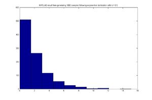
MATLAB code

for exponential distribution case,assuming [math]\displaystyle{ \lambda=0.5 }[/math]

for ii = 1:1000
    u = rand;
    x(ii) = -log(1-u)/0.5;
end
hist(x)

MATLAB result

Discrete Case - September 22, 2011

This same technique can be applied to the discrete case. Generate a discrete random variable [math]\displaystyle{ \,x }[/math] that has probability mass function [math]\displaystyle{ \,P(X=x_i)=P_i }[/math] where [math]\displaystyle{ \,x_0\lt x_1\lt x_2... }[/math] and [math]\displaystyle{ \,\sum_i P_i=1 }[/math]

• Step 1. Draw [math]\displaystyle{ u \sim~ \mathrm{Unif}[0, 1] }[/math]
• Step 2. [math]\displaystyle{ \,x=x_i }[/math] if [math]\displaystyle{ \,F(x_{i-1})\lt u \leq F(x_i) }[/math]

Example

Let x be a discrete random variable with the following probability mass function:

[math]\displaystyle{ \begin{align} P(X=0) = 0.3 \\ P(X=1) = 0.2 \\ P(X=2) = 0.5 \end{align} }[/math]

Given the pmf, we now need to find the cdf.

We have:

[math]\displaystyle{ F(x) = \begin{cases} 0 & x \lt 0 \\ 0.3 & 0 \leq x \lt 1 \\ 0.5 & 1 \leq x \lt 2 \\ 1 & 2 \leq x \end{cases} }[/math]

We can apply the inverse transform method to obtain our random numbers from this distribution.

Pseudo Code for generating the random numbers:

Draw U ~ Unif[0,1] 
if U <= 0.3 
  return 0 
else if 0.3 < U <= 0.5 
  return 1
else if 0.5 < U <= 1 
  return 2

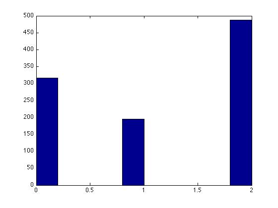
MATLAB code for generating 1000 random numbers in the discrete case:

for ii = 1:1000
  u = rand;
    
  if u <= 0.3
    x(ii) = 0;
  else if u <= 0.5
    x(ii) = 1;
  else
    x(ii) = 2;
  end
end

Matlab Output:

Pseudo code for the Discrete Case:

1. Draw U ~ Unif [0,1]

2. If [math]\displaystyle{ U \leq P_0 }[/math], deliver X= x₀

3. Else if [math]\displaystyle{ U \leq P_0 + P_1 }[/math], deliver X= x₁

4. Else If [math]\displaystyle{ U \leq P_0 +....+ P_k }[/math], deliver X= x_k

Limitations

Although this method is useful, it isn't practical in many cases since we can't always obtain [math]\displaystyle{ F }[/math] or [math]\displaystyle{ F^{-1} }[/math] as some functions are not integrable or invertible, and sometimes even [math]\displaystyle{ f(x) }[/math] itself cannot be obtained in closed form. Let's look at some examples:

• Continuous case

If we want to use this method to draw the pdf of normal distribution, we may find ourselves get stuck in finding its cdf. The simplest case of normal distribution is [math]\displaystyle{ f(x)=\frac{1}{\sqrt{2\pi}}e^{-\frac{x^2}{2}} }[/math], whose cdf is [math]\displaystyle{ F(x)=\frac{1}{\sqrt{2\pi}}\int_{-\infty}^{x}{e^{-\frac{u^2}{2}}}du }[/math]. This integral cannot be expressed in terms of elementary functions. So evaluating it and then finding the inverse is a very difficult task.

• Discrete case

It is easy for us to simulate when there are only a few values taken by the particular random variable, like the case above. And it is easy to simulate the binomial distribution [math]\displaystyle{ X \sim~ \mathrm{B}(n,p) }[/math] when the parameter n is not too large. But when n takes on values that are very large, say 50, it is hard to do so.

Acceptance/Rejection Method

The aforementioned difficulties of the inverse transform method motivates a sampling method that does not require analytically calculating cdf's and their inverses, which is the acceptance/rejection sampling method. Here, [math]\displaystyle{ \displaystyle f(x) }[/math] is approximated by another function, say [math]\displaystyle{ \displaystyle g(x) }[/math], with the idea being that [math]\displaystyle{ \displaystyle g(x) }[/math] is a "nicer" function to work with than [math]\displaystyle{ \displaystyle f(x) }[/math].

Suppose we assume the following:

1. There exists another distribution [math]\displaystyle{ \displaystyle g(x) }[/math] that is easier to work with and that you know how to sample from, and

2. There exists a constant c such that [math]\displaystyle{ f(x) \leq c \cdot g(x) }[/math] for all x

Under these assumptions, we can sample from [math]\displaystyle{ \displaystyle f(x) }[/math] by sampling from [math]\displaystyle{ \displaystyle g(x) }[/math]

General Idea

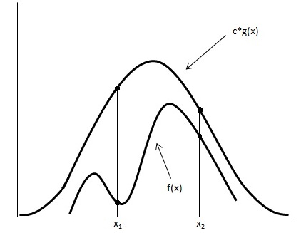
Looking at the image below we have graphed [math]\displaystyle{ c \cdot g(x) }[/math] and [math]\displaystyle{ \displaystyle f(x) }[/math].

Using the acceptance/rejection method we will accept some of the points from [math]\displaystyle{ \displaystyle g(x) }[/math] and reject some of the points from [math]\displaystyle{ \displaystyle g(x) }[/math]. The points that will be accepted from [math]\displaystyle{ \displaystyle g(x) }[/math] will have a distribution similar to [math]\displaystyle{ \displaystyle f(x) }[/math]. We can see from the image that the values around [math]\displaystyle{ \displaystyle x_1 }[/math] will be sampled more often under [math]\displaystyle{ c \cdot g(x) }[/math] than under [math]\displaystyle{ \displaystyle f(x) }[/math], so we will have to reject more samples taken at x₁. Around [math]\displaystyle{ \displaystyle x_2 }[/math] the number of samples that are drawn and the number of samples we need are much closer, so we accept more samples that we get at [math]\displaystyle{ \displaystyle x_2 }[/math]

Procedure

1. Draw y ~ g

2. Draw U ~ Unif [0,1]

3. If [math]\displaystyle{ U \leq \frac{f(y)}{c \cdot g(y)} }[/math] then x=y; else return to 1

Proof

Mathematically, we need to show that the sample points given that they are accepted have a distribution of f(x).

[math]\displaystyle{ \begin{align} P(y|accepted) &= \frac{P(y, accepted)}{P(accepted)} \\ &= \frac{P(accepted|y) P(y)}{P(accepted)}\end{align} }[/math] (Bayes' Rule)

[math]\displaystyle{ \displaystyle P(y) = g(y) }[/math]

[math]\displaystyle{ P(accepted|y) =P(u\leq \frac{f(y)}{c \cdot g(y)}) =\frac{f(y)}{c \cdot g(y)} }[/math],where u ~ Unif [0,1]

[math]\displaystyle{ P(accepted) = \sum P(accepted|y)\cdot P(y)=\int^{}_y \frac{f(y)}{c \cdot g(y)}g(y) dy=\int^{}_y \frac{f(y)}{c} dy=\frac{1}{c} \cdot\int^{}_y f(y) dy=\frac{1}{c} }[/math]

So,

[math]\displaystyle{ P(y|accepted) = \frac{ \frac {f(y)}{c \cdot g(y)} \cdot g(y)}{\frac{1}{c}} =f(y) }[/math]

Continuous Case

Example

Sample from Beta(2,1)

In general:

Beta([math]\displaystyle{ \alpha, \beta) = \frac{\Gamma (\alpha + \beta)}{\Gamma(\alpha)\Gamma(\beta)} }[/math] [math]\displaystyle{ \displaystyle x^{\alpha-1} }[/math] [math]\displaystyle{ \displaystyle(1-x)^{\beta-1} }[/math], [math]\displaystyle{ \displaystyle 0\lt x\lt 1 }[/math]

Note: [math]\displaystyle{ \!\Gamma(n) = (n-1)! }[/math] if n is a positive integer

[math]\displaystyle{ \begin{align} f(x) &= Beta(2,1) \\ &= \frac{\Gamma(3)}{\Gamma(2)\Gamma(1)} x^1(1-x)^0 \\ &= \frac{2!}{1! 0!}\cdot (1) x \\ &= 2x \end{align} }[/math]

We want to choose [math]\displaystyle{ \displaystyle g(x) }[/math] that is easy to sample from. So we choose [math]\displaystyle{ \displaystyle g(x) }[/math] to be uniform distribution.

We now want a constant c such that [math]\displaystyle{ f(x) \leq c \cdot g(x) }[/math] for all x from Unif(0,1)

So,

[math]\displaystyle{ c \geq \frac{f(x)}{g(x)} }[/math], for all x from (0,1)

[math]\displaystyle{ \begin{align}c &\geq max (\frac {f(x)}{g(x)}, 0\lt x\lt 1) \\ &= max (\frac {2x}{1},0\lt x\lt 1) \\ &= 2 \end{align} }[/math]

Now that we have c =2,

1. Draw y ~ g(x) => Draw y ~ Unif [0,1]

2. Draw u ~ Unif [0,1]

3. if [math]\displaystyle{ u \leq \frac{2y}{2 \cdot 1} }[/math] then x=y; else return to 1

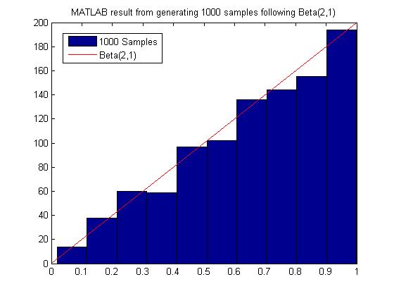
MATLAB code for generating 1000 samples following Beta(2,1):

close all
clear all
ii=1;
while ii < 1000
    y = rand;
    u = rand;
    
    if u <= y
        x(ii)=y;
        ii=ii+1;
    end
end
hist(x)

MATLAB result

Discrete Example

Generate random variables according to the p.m.f:

[math]\displaystyle{ \begin{align} P(Y=1) = 0.15 \\ P(Y=2) = 0.22 \\ P(Y=3) = 0.33 \\ P(Y=4) = 0.10 \\ P(Y=5) = 0.20 \end{align} }[/math]

find a g(y) discrete uniform distribution from 1 to 5

[math]\displaystyle{ c \geq \frac{P(y)}{g(y)} }[/math]
[math]\displaystyle{ c = \max \left(\frac{P(y)}{g(y)} \right) }[/math]
[math]\displaystyle{ c = \max \left(\frac{0.33}{0.2} \right) = 1.65 }[/math] Since P(Y=3) is the max of P(Y) and g(y) = 0.2 for all y.

1. Generate Y according to the discrete uniform between 1 - 5

2. U ~ unif[0,1]

3. If [math]\displaystyle{ U \leq \frac{P(y)}{1.65 \times 0.2} \leq \frac{P(y)}{0.33} }[/math], then x = y; else return to 1.

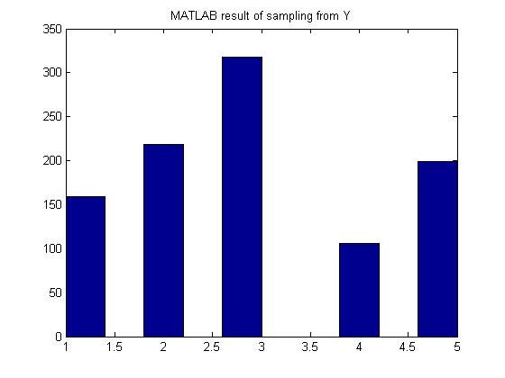
In MATLAB, the code would be:

   py = [0.15 0.22 0.33 0.1 0.2];
   ii =1;
   while ii <= 1000
       y = unidrnd(5);
       u = rand;
       if u <= py(y)/0.33
           x(ii) = y;
           ii = ii+1;
       end
   end
   hist(x);

MATLAB result

Limitations

Most of the time we have to sample many more points from g(x) before we can obtain an acceptable amount of samples from f(x), hence this method may not be computationally efficient. It depends on our choice of g(x). For example, in the example above to sample from Beta(2,1), we need roughly 2000 samples from g(X) to get 1000 acceptable samples of f(x).

In addition, in situations where a g(x) function is chosen and used, there can be a discrepancy between the functional behaviors of f(x) and g(x) that render this method unreliable. For example, given the normal distribution function as g(x) and a function of f(x) with a "fat" mid-section and "thin tails", this method becomes useless as more points near the two ends of f(x) will be rejected, resulting in a tedious and overwhelming number of sampling points having to be sampled due to the high rejection rate of such a method.

Sampling From Gamma and Normal Distribution - September 27, 2011

Sampling From Gamma

Gamma Distribution

The Gamma function is written as [math]\displaystyle{ X \sim~ Gamma (t, \lambda) }[/math]

[math]\displaystyle{ F(x) = \int_{0}^{\lambda x} \frac{e^{-y}y^{t-1}}{(t-1)!} dy }[/math]

If you have t samples of the exponential distribution,

[math]\displaystyle{ \begin{align} X_1 \sim~ Exp(\lambda)\\ \vdots \\ X_t \sim~ Exp(\lambda) \end{align} }[/math]

The sum of these t samples has a gamma distribution,

[math]\displaystyle{ X_1+X_2+ ... + X_t \sim~ Gamma (t, \lambda) }[/math]

[math]\displaystyle{ \sum_{i=1}^{t} X_i \sim~ Gamma (t, \lambda) }[/math] where [math]\displaystyle{ X_i \sim~Exp(\lambda) }[/math]

Method

We can sample the exponential distribution using the inverse transform method from previous class,

[math]\displaystyle{ \,f(x)={\lambda}e^{-{\lambda}x} }[/math]

[math]\displaystyle{ \,F^{-1}(u)=\frac{-ln(1-u)}{\lambda} }[/math]

[math]\displaystyle{ \,F^{-1}(u)=\frac{-ln(u)}{\lambda} }[/math]

1 - u is the same as x since [math]\displaystyle{ U \sim~ unif [0,1] }[/math]

[math]\displaystyle{ \begin{align} \frac{-ln(u_1)}{\lambda} - \frac{ln(u_2)}{\lambda} - ... - \frac{ln(u_t)}{\lambda} = x_1\\ \vdots \\ \frac{-ln(u_1)}{\lambda} - \frac{ln(u_2)}{\lambda} - ... - \frac{ln(u_t)}{\lambda} = x_t \end{align}  : }[/math]

[math]\displaystyle{ \frac {-\sum_{i=1}^{t} ln(u_i)}{\lambda} = x }[/math]

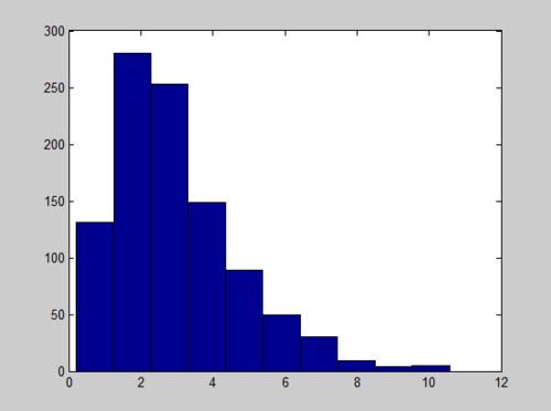
MATLAB code for a Gamma(1,3) is

x = sum(-log(rand(1000,3)),2); 
hist(x)

And the Histogram of X follows a Gamma distribution with long tail:

We can improve the quality of histogram by adding the number of bins we want, like hist(x, number_of_bins)

x = sum(-log(rand(20000,3)),2); 
hist(x,40)

File:untitled.jpg

R code for a Gamma(1,3) is

a<-apply(-log(matrix(runif(3000),nrow=1000)),1,sum);
hist(a);

And the histogram is

File:hist gamma.png

Here is another histogram of Gamma coding with R

a<-apply(-log(matrix(runif(3000),nrow=1000)),1,sum);
hist(a,freq=F);
lines(density(a),col="blue");
rug(jitter(a));

File:hist gamma 2.png

Sampling from Normal Distribution using Box-Muller Transform - September 29, 2011

Procedure

1. Generate [math]\displaystyle{ \displaystyle u_1 }[/math] and [math]\displaystyle{ \displaystyle u_2 }[/math], two values sampled from a uniform distribution between 0 and 1.
2. Set [math]\displaystyle{ \displaystyle R^2 = -2log(u_1) }[/math] so that [math]\displaystyle{ \displaystyle R^2 }[/math] is exponential with mean 1/2
   Set [math]\displaystyle{ \!\theta = 2*\pi*u_2 }[/math] so that [math]\displaystyle{ \!\theta }[/math] ~ Unif[0, 2[math]\displaystyle{ \displaystyle\pi }[/math]]
3. Set [math]\displaystyle{ \displaystyle X = R cos(\theta) }[/math]
   Set [math]\displaystyle{ \displaystyle Y = R sin(\theta) }[/math]

Justification

Suppose we have X ~ N(0, 1) and Y ~ N(0, 1) where X and Y are independent normal random variables. The relative probability density function of these two random variables using Cartesian coordinates is:

[math]\displaystyle{ f(X, Y) dxdy= f(X) f(Y) dxdy= \frac{1}{\sqrt{2\pi}}e^{-x^2/2} \frac{1}{\sqrt{2\pi}}e^{-y^2/2} dxdy= \frac{1}{2\pi}e^{-(x^2+y^2)/2}dxdy }[/math]

In polar coordinates [math]\displaystyle{ \displaystyle R^2 = x^2 + y^2 }[/math], so the relative probability density function of these two random variables using polar coordinates is:

[math]\displaystyle{ f(R, \theta) = \frac{1}{2\pi}e^{-R^2/2} }[/math]

If we have [math]\displaystyle{ \displaystyle R^2 \sim exp(1/2) }[/math] and [math]\displaystyle{ \!\theta \sim unif[0, 2\pi] }[/math] we get an equivalent relative probability density function. Notice that after the two on two transformation, a determinant of jocobian should be added according to the change of variable and rule of differential multiplication where

[math]\displaystyle{ |J|=\left|\frac{\partial(x,y)}{\partial(R,\theta)}\right|= \left|\begin{matrix}\frac{\partial x}{\partial R}&\frac{\partial x}{\partial \theta}\\\frac{\partial y}{\partial R}&\frac{\partial y}{\partial \theta}\end{matrix}\right|=R }[/math]

[math]\displaystyle{ f(X, Y) dxdy = f(R, \theta)|J|dRd\theta = \frac{1}{2\pi}e^{-R^2/2}R dRd\theta= \frac{1}{4\pi}e^{-\frac{s}{2}} dSd\theta }[/math]
where [math]\displaystyle{ S=R^2. }[/math]

Therefore we can generate a point in polar coordinates using the uniform and exponential distributions, then convert the point to Cartesian coordinates and the resulting X and Y values will be equivalent to samples generated from N(0, 1).

MATLAB code

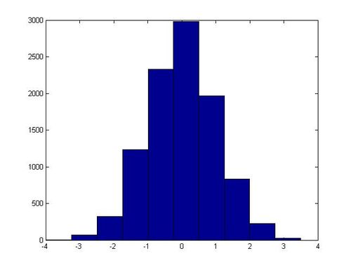
In MatLab this algorithm can be implemented with the following code, which generates 20,000 samples from N(0, 1):

x = zeros(10000, 1);
y = zeros(10000, 1);
for ii = 1:10000
    u1 = rand;
    u2 = rand;
    R2 = -2 * log(u1);
    theta = 2 * pi * u2;
    x(ii) = sqrt(R2) * cos(theta);
    y(ii) = sqrt(R2) * sin(theta);
end
hist(x)

In one execution of this script, the following histogram for x was generated:

Non-Standard Normal Distributions

Example 1: Single-variate Normal

If X ~ Norm(0, 1) then (a + bX) has a normal distribution with a mean of [math]\displaystyle{ \displaystyle a }[/math] and a standard deviation of [math]\displaystyle{ \displaystyle b }[/math] (which is equivalent to a variance of [math]\displaystyle{ \displaystyle b^2 }[/math]). Using this information with the Box-Muller transform, we can generate values sampled from some random variable [math]\displaystyle{ \displaystyle Y\sim N(a,b^2) }[/math] for arbitrary values of [math]\displaystyle{ \displaystyle a,b }[/math].

1. Generate a sample u from Norm(0, 1) using the Box-Muller transform.
2. Set v = a + bu.

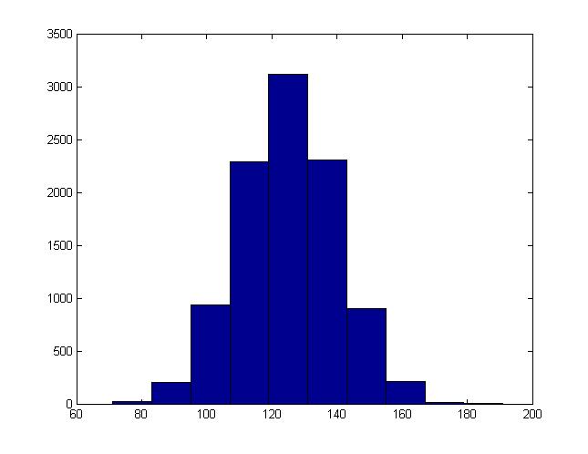
The values for v generated in this way will be equivalent to sample from a [math]\displaystyle{ \displaystyle N(a, b^2) }[/math]distribution. We can modify the MatLab code used in the last section to demonstrate this. We just need to add one line before we generate the histogram:

x = a + b * x;

For instance, this is the histogram generated when b = 15, a = 125:

500

Example 2: Multi-variate Normal

The Box-Muller method can be extended to higher dimensions to generate multivariate normals. The objects generated will be nx1 vectors, and their variance will be described by nxn covariance matrices.

[math]\displaystyle{ \mathbf{z} = N(\mathbf{u}, \Sigma) }[/math] defines the n by 1 vector [math]\displaystyle{ \mathbf{z} }[/math] such that:

• [math]\displaystyle{ \displaystyle u_i }[/math] is the average of [math]\displaystyle{ \displaystyle z_i }[/math]
• [math]\displaystyle{ \!\Sigma_{ii} }[/math] is the variance of [math]\displaystyle{ \displaystyle z_i }[/math]
• [math]\displaystyle{ \!\Sigma_{ij} }[/math] is the co-variance of [math]\displaystyle{ \displaystyle z_i }[/math] and [math]\displaystyle{ \displaystyle z_j }[/math]

If [math]\displaystyle{ \displaystyle z_1, z_2, ..., z_d }[/math] are normal variables with mean 0 and variance 1, then the vector [math]\displaystyle{ \displaystyle (z_1, z_2,..., z_d) }[/math] has mean 0 and variance [math]\displaystyle{ \!I }[/math], where 0 is the zero vector and [math]\displaystyle{ \!I }[/math] is the identity matrix. This fact suggests that the method for generating a multivariate normal is to generate each component individually as single normal variables.

The mean and the covariance matrix of a multivariate normal distribution can be adjusted in ways analogous to the single variable case. If [math]\displaystyle{ \mathbf{z} \sim N(0,I) }[/math], then [math]\displaystyle{ \Sigma^{1/2}\mathbf{z}+\mu \sim N(\mu,\Sigma) }[/math]. Note here that the covariance matrix is symmetric and nonnegative, so its square root should always exist.

We can compute [math]\displaystyle{ \mathbf{z} }[/math] in the following way:

1. Generate an n by 1 vector [math]\displaystyle{ \mathbf{x} = \begin{bmatrix}x_{1} & x_{2} & ... & x_{n}\end{bmatrix} }[/math] where [math]\displaystyle{ x_{i} }[/math] ~ Norm(0, 1) using the Box-Muller transform.
2. Calculate [math]\displaystyle{ \!\Sigma^{1/2} }[/math] using singular value decomposition.
3. Set [math]\displaystyle{ \mathbf{z} = \Sigma^{1/2} \mathbf{x} + \mathbf{u} }[/math].

The following MatLab code provides an example, where a scatter plot of 10000 random points is generated. In this case x and y have a co-variance of 0.9 - a very strong positive correlation.

x = zeros(10000, 1);
y = zeros(10000, 1);
for ii = 1:10000
    u1 = rand;
    u2 = rand;
    R2 = -2 * log(u1);
    theta = 2 * pi * u2;
    x(ii) = sqrt(R2) * cos(theta);
    y(ii) = sqrt(R2) * sin(theta);
end

E = [1, 0.9; 0.9, 1];
[u s v] = svd(E);
root_E = u * (s ^ (1 / 2));

z = (root_E * [x y]);
z(:,1) = z(:,1) + 5;
z(:,2) = z(:,2) + -8;

scatter(z(:,1), z(:,2))

This code generated the following scatter plot:

File:scatter covar.jpg

In Matlab, we can also use the function "sqrtm()" to calculate Square root of a matrix directly. Here is an example:

E = [1, 0.9; 0.9, 1];
sqrtm(E);

R code for a multivariate normal distribution:

n=10000;
r2<--2*log(runif(n));
theta<-2*pi*(runif(n));
x<-sqrt(r2)*cos(theta);

y<-sqrt(r2)*sin(theta);
a<-matrix(c(x,y),nrow=n,byrow=F);
e<-matrix(c(1,.9,09,1),nrow=2,byrow=T);
svde<-svd(e);
root_e<-svde$u %*% diag(svde$d)^1/2;
z<-t(root_e %*%t(a));
z[,1]=z[,1]+5;
z[,2]=z[,2]+ -8;
par(pch=19);
plot(z,col=rgb(1,0,0,alpha=0.06))

File:m normal.png

Remarks

MATLAB's randn function uses the ziggurat method to generate normal distributed samples. It is an efficient rejection method based on covering the probability density function with a set of horizontal rectangles so as to obtain points within each rectangle. It is reported that a 800 MHz Pentium III laptop can generate over 10 million random numbers from normal distribution in less than one second. (Reference)

Sampling From Binomial Distributions

In order to generate a sample x from [math]\displaystyle{ \displaystyle X \sim Bin(n, p) }[/math], we can follow the following procedure:

1. Generate n uniform random numbers sampled from [math]\displaystyle{ \displaystyle Unif [0, 1] }[/math]: [math]\displaystyle{ \displaystyle u_1, u_2, ..., u_n }[/math].

2. Set x to be the total number of cases where [math]\displaystyle{ \displaystyle u_i \lt = p }[/math] for all [math]\displaystyle{ \displaystyle 1 \lt = i \lt = n }[/math].

In MatLab this can be coded with a single line. The following generates a sample from [math]\displaystyle{ \displaystyle X \sim Bin(n, p) }[/math]

>> sum(rand(n, 1) <= p, 1)

Bayesian Inference and Frequentist Inference - October 4, 2011

Bayesian inference vs Frequentist inference

The Bayesian method has become popular in the last few decades as simulation and computer technology makes it more applicable. For more information about its history and application, please refer to http://en.wikipedia.org/wiki/Bayesian_inference. As for frequentists, please refer to http://en.wikipedia.org/wiki/Frequentist_inference.

Example

Consider: A person drinks a cup of coffee on a specific day.

Frequentist: There is no explanation to this situation. It is essentially meaningless since it has only occurred once. Therefore, it is not a probability.
Bayesian: Probability is not just about the frequent occurrences but it is what you believe about this probability.

Example of face identification

Take the face as input x. And the person as output y. The person can be either Ali or Tom. If it is Ali, y=1. Otherwise, y=0. We can divide the picture into 100*100 pixels and then list them into a 10,000*1 column vector which is x.

If you are a frequentist, you would compare Pr(X=x|y=1) with Pr(X=x|y=0) and see which one is higher. But if you are a Bayesianist, you would compare Pr(y=1|X=x) with Pr(y=0|X=x).

Summary of differences between two schools

• Frequentist: Probability refers to limiting relative frequency. (objective)
• Bayesian: Probability describes degree of belief not frequency. (subjective)

e.g. The probability that you drank a cup of tea on May 20, 2001 is 0.62 does not refer to any frequency.

---

• Frequentist: Parameters are fixed, unknown constants.
• Bayesian: Parameters are random variables and we can make probabilistic statement about them.

---

• Frequentist: Statistical procedures should have long run frequency probabilities.

e.g. a 95% confidence interval should trap true value of the parameter for at least 95% of limited frequency

• Bayesian: It makes inferences about [math]\displaystyle{ \theta }[/math] by producing a prbability distribution for [math]\displaystyle{ \theta }[/math]. Inference (e.g. point estimation) will be extracted from this distribution.

Bayesian inference

Bayesian inference is usually carried out in the following way:

1. Choose a prior probability density function of [math]\displaystyle{ \!\theta }[/math] which is [math]\displaystyle{ f(\!\theta) }[/math]. This is our belief about [math]\displaystyle{ \theta }[/math] before we see any data.

2. Choose a statistical model [math]\displaystyle{ \displaystyle f(x|\theta) }[/math] that reflects our beliefs about X.

3. After observing data [math]\displaystyle{ \displaystyle x_1,...,x_n }[/math], we update our beliefs and calculate the posterior probability.

[math]\displaystyle{ f(\theta|x) = \frac{f(\theta,x)}{f(x)}=\frac{f(x|\theta) \cdot f(\theta)}{f(x)}=\frac{f(x|\theta) \cdot f(\theta)}{\int^{}_\theta f(x|\theta) \cdot f(\theta) d\theta} }[/math], where [math]\displaystyle{ \displaystyle f(\theta|x) }[/math] is the posterior probability, [math]\displaystyle{ \displaystyle f(\theta) }[/math] is the prior probability, [math]\displaystyle{ \displaystyle f(x|\theta) }[/math] is the likelihood of observing X=x given [math]\displaystyle{ \!\theta }[/math] and f(x) is the marginal probability of X=x.

If we have i.i.d. observations [math]\displaystyle{ \displaystyle x_1,...,x_n }[/math], we can replace [math]\displaystyle{ \displaystyle f(x|\theta) }[/math] with [math]\displaystyle{ f({x_1,...,x_n}|\theta)=\prod_{i=1}^n f(x_i|\theta) }[/math] because of independency.

We denote [math]\displaystyle{ \displaystyle f({x_1,...,x_n}|\theta) }[/math] as [math]\displaystyle{ \displaystyle L_n(\theta) }[/math] which is called likelihood. And we use [math]\displaystyle{ \displaystyle x^n }[/math] to denote [math]\displaystyle{ \displaystyle (x_1,...,x_n) }[/math].

[math]\displaystyle{ f(\theta|x^n) = \frac{f(x^n|\theta) \cdot f(\theta)}{f(x^n)}=\frac{f(x^n|\theta) \cdot f(\theta)}{\int^{}_\theta f(x^n|\theta) \cdot f(\theta) d\theta} }[/math] , where [math]\displaystyle{ \int^{}_\theta f(x^n|\theta) \cdot f(\theta) d\theta }[/math] is a constant [math]\displaystyle{ \displaystyle c_n }[/math]. So [math]\displaystyle{ f(\theta|x^n) \propto f(x^n|\theta) \cdot f(\theta) }[/math]. The posterior probability is proportional to the likelihood times prior probability.

[math]\displaystyle{ E(\theta)=\int^{}_\theta \theta \cdot f(\theta|x^n) d\theta }[/math] which is the posterior mean of [math]\displaystyle{ \!\theta }[/math].

Let [math]\displaystyle{ \tilde{\theta}=(\theta_1,...,\theta_d)^T }[/math], then [math]\displaystyle{ f(\theta_1|x^n) = \int^{} \int^{} \dots \int^{}f(\theta|X)d\theta_2d\theta_3 \dots d\theta_d }[/math] and [math]\displaystyle{ E(\theta_1)=\int^{}\theta_1 \cdot f(\theta_1|x^n) d\theta_1 }[/math]

Example 1: Estimating parameters of a univariate Gaussian distribution

Suppose X follows a univariate Gaussian distribution (i.e. a Normal distribution) with parameters [math]\displaystyle{ \!\mu }[/math] and [math]\displaystyle{ \displaystyle {\sigma^2} }[/math].

(a) For Frequentists:

[math]\displaystyle{ f(x|\theta)= \frac{1}{\sqrt{2\pi}\sigma} \cdot e^{-\frac{1}{2}(\frac{x-\mu}{\sigma})^2} }[/math]

[math]\displaystyle{ L_n(\theta)= \prod_{i=1}^n \frac{1}{\sqrt{2\pi}\sigma} \cdot e^{-\frac{1}{2}(\frac{x_i-\mu}{\sigma})^2} }[/math]

[math]\displaystyle{ \ln L_n(\theta) = l(\theta) = \sum_{i=1}^n -\frac{1}{2}\ln 2\pi-\ln \sigma-\frac{1}{2}(\frac{x_i-\mu}{\sigma})^2 }[/math]

To get the maximum likelihood estimator of [math]\displaystyle{ \!\mu }[/math] (mle), we find the [math]\displaystyle{ \hat{\mu} }[/math] which maximizes [math]\displaystyle{ \displaystyle L_n(\theta) }[/math]:

[math]\displaystyle{ \frac{\partial l(\theta)}{\partial \mu}= \sum_{i=1}^n \frac{1}{\sigma}(\frac{x_i-\mu}{\sigma})=0 \Rightarrow \sum_{i=1}^n x_i = n\mu \Rightarrow \hat{\mu}_{mle}=\bar{x} }[/math]

(b) For Bayesians:

[math]\displaystyle{ f(\theta|x) \propto f(x|\theta) \cdot f(\theta) }[/math]

We assume that the mean of the above normal distribution is itself distributed normally with mean [math]\displaystyle{ \!\mu_0 }[/math] and variance [math]\displaystyle{ \!\Gamma }[/math].

Suppose [math]\displaystyle{ \!\mu\sim N(\mu_0, \!\Gamma^2 }[/math]),

so [math]\displaystyle{ f(\mu) = \frac{1}{\sqrt{2\pi}\Gamma} \cdot e^{-\frac{1}{2}(\frac{\mu-\mu_0}{\Gamma})^2} }[/math]

[math]\displaystyle{ f(\mu|x) = \frac{1}{\sqrt{2\pi}\tilde{\sigma}} \cdot e^{-\frac{1}{2}(\frac{\mu-\tilde{\mu}}{\tilde{\sigma}})^2} }[/math]

[math]\displaystyle{ \tilde{\mu} = \frac{\frac{n}{\sigma^2}}{\frac{n}{\sigma^2}+\frac{1}{\Gamma^2}}\bar{x}+\frac{\frac{1}{\Gamma^2}}{\frac{n}{\sigma^2}+\frac{1}{\Gamma^2}}\mu_0 }[/math], where [math]\displaystyle{ \tilde{\mu} }[/math] is the estimator of [math]\displaystyle{ \!\mu }[/math].

• If prior belief about [math]\displaystyle{ \!\mu_0 }[/math] is strong, then [math]\displaystyle{ \!\Gamma }[/math] is small and [math]\displaystyle{ \frac{1}{\Gamma^2} }[/math] is large. [math]\displaystyle{ \tilde{\mu} }[/math] is close to [math]\displaystyle{ \!\mu_0 }[/math] and the observations will not affect too much. On the contrary, if prior belief about [math]\displaystyle{ \!\mu_0 }[/math] is weak, [math]\displaystyle{ \!\Gamma }[/math] is large and [math]\displaystyle{ \frac{1}{\Gamma^2} }[/math] is small. [math]\displaystyle{ \tilde{\mu} }[/math] depends more on observations.(This is intuitive, when our original belief is reliable, then the sample is not important in improving the result; when the belief is not reliable, then we depend a lot on the sample.)

• When the sample is large (i.e. n [math]\displaystyle{ \to \infty }[/math]), [math]\displaystyle{ \tilde{\mu} \to \bar{x} }[/math] and the impact of prior belief about [math]\displaystyle{ \!\mu }[/math] is weakened.

Basic Monte Carlo Integration - October 6th, 2011

Three integration methods would be taught in this course:

• Basic Monte Carlo Integration
• Importance Sampling
• Markov Chain Monte Carlo (MCMC)

The first, and most basic, method of numerical integration we will see is Monte Carlo Integration. We use this to solve an integral of the form: [math]\displaystyle{ I = \int_{a}^{b} h(x) dx }[/math]

Note the following derivation:

[math]\displaystyle{ \begin{align} \displaystyle I & = \int_{a}^{b} h(x)dx \\ & = \int_{a}^{b} h(x)((b-a)/(b-a))dx \\ & = \int_{a}^{b} (h(x)(b-a))(1/(b-a))dx \\ & = \int_{a}^{b} w(x)f(x)dx \\ & = E[w(x)] \\ \end{align} }[/math]

~[math]\displaystyle{ (1/n) \sum_{i=1}^{n} w(x) }[/math]

Where w(x) = h(x)(b-a) and f(x) is the probability density function of a uniform random variable on the interval [a,b]. The expectation, with respect to the distribution of f, of w is taken from n samples of x.

General Procedure

i) Draw n samples x_i ~ uniform[a,b]

ii) Compute w(x_i)

        [math]\displaystyle{  \hat{I} = 1/n \sum_{i=1}^{n} w(x }[/math]i[math]\displaystyle{  ) }[/math]

By the strong law of large numbers I^{^} converges to I as n approaches [math]\displaystyle{ \infty }[/math]. Because of this, we can compute all sorts of useful information, such as variance, standard error, and confidence intervals.

Standard Error: [math]\displaystyle{ SE = Standard Deviation / \sqrt{n} }[/math]

Variance: [math]\displaystyle{ V = (\sum_{i=1}^{n} (w(x)-I)^2)/(n-1) }[/math]

Confidence Interval: [math]\displaystyle{ I \pm t_{(\alpha/2)} SE }[/math]

Example: Uniform Distribution

Consider the integral, [math]\displaystyle{ \int_{0}^{1} x^3dx }[/math], which is easily solved through standard analytical integration methods, and is equal to .25. Now, let us check this answer with a numerical approximation using Monte Carlo Integration.

We generate a 1 by 10000 vector of uniform (on the interval [0,1]) random variables and call that vector 'u'. We see that our 'w' in this case is [math]\displaystyle{ x^3 }[/math], so we set [math]\displaystyle{ w = u^3 }[/math]. Our I^{^} is equal to the mean of w.

In Matlab, we can solve this integration problem with the following code:

u = rand(1,10000);
w = u.^3;
mean(w)
  ans = 0.2475

Note the '.' after 'u' in the second line of code, indicating that each entry in the matrix is cubed. Also, our approximation is close to the actual value of .25. Now let's try to get an even better approximation by generating more sample points.

u= rand(1,100000);
w= u.^3;
mean(w)
  ans = .2503

We see that when the number of sample points is increased, our approximation improves, as one would expect.

Generalization

Up to this point we have seen how to numerically approximate an integral when the distribution of f is uniform. Now we will see how to generalize this to other distributions.

[math]\displaystyle{ I = \int h(x)f(x)dx }[/math]

If f is a distribution function (pdf), then [math]\displaystyle{ I }[/math] can be estimated as E_f[h(x)]. This means taking the expectation of h with respect to the distribution of f. Our previous example is the case where f is the uniform distribution between [a,b].

Procedure for the General Case

i) Draw n samples from f

ii) Compute h(x_i)

iii) [math]\displaystyle{ \hat{I} = 1/n \sum_{i=1}^{n} h(x }[/math]_i[math]\displaystyle{ ) }[/math]

Example: Exponential Distribution

Find [math]\displaystyle{ E[\sqrt{x}] }[/math] for [math]\displaystyle{ \displaystyle f = e^{-x} }[/math], which is the exponential distribution with mean 1.

[math]\displaystyle{ I = \int_{0}^{\infty} \sqrt{x} e^{-x}dx }[/math]

We can see that we must draw samples from f, the exponential distribution.

To find a numerical solution using Monte Carlo Integration we see that:

u= rand(1,10000) X= -log(u) h= [math]\displaystyle{ \sqrt{x} }[/math] I= mean(h)

To implement this procedure in Matlab, use the following code:

u = rand(1,10000);
X = -log(u);
h = x.^.5;
mean(h)
  ans = .8841

An easy way to check whether your approximation is correct is to use the built in Matlab function 'quadl' which takes a function and bounds for the integral and returns a solution for the definite integral of that function. For this specific example, we can enter:

f = @(x) sqrt(x).*exp(-x);
% quadl runs into computational problems when the upper bound is "inf" or an extremely large number, 
% so choose just a moderately large number.
quadl(f,0,100)
ans =
  0.8862

From the above result, we see that our approximation was quite close.

Example: Normal Distribution

Let [math]\displaystyle{ f(x) = (1/(2 \pi)^{1/2}) e^{(-x^2)/2} }[/math]. Compute the cumulative distribution function at some point x.

[math]\displaystyle{ F(x)= \int_{-\infty}^{x} f(s)ds = \int_{-\infty}^{x}(1)(1/(2 \pi)^{1/2}) e^{(-s^2)/2}ds }[/math]. The (1) is inserted to illustrate that our h(x) will be the constant function 1, and our f(x) is the normal distribution. To take into account the upper bound of integration, x, any values sampled that are greater than x will be set to zero.

This is the Matlab code for solving F(2):

u = randn(1,10000)
h = u < 2;
mean(h)
  ans = .9756

We generate a 1 by 10000 vector of standard normal random variables and we return a value of 1 if u is less than 2, and 0 otherwise.

We can also build the function F(x) in matlab in the following way:

function F(x)
u=rand(1,1000000);
h=u<x;
mean(h)

Example: Binomial Distribution

In this example we will see the Bayesian Inference for 2 Binomial Distributions.

Let [math]\displaystyle{ X ~ Bin(n,p) }[/math] and [math]\displaystyle{ Y ~ Bin(m,q) }[/math], and let [math]\displaystyle{ \!\delta = p-q }[/math].

Therefore, [math]\displaystyle{ \displaystyle \!\delta = x/n - y/m }[/math] which is the frequentist approach.

Bayesian wants [math]\displaystyle{ \displaystyle f(p,q|x,y) = f(x,y|p,q)f(p,q)/f(x,y) }[/math], where [math]\displaystyle{ f(x,y)=\iint\limits_{\!\theta} f(x,y|p,q)f(p,q)\,dp\,dq }[/math] is a constant.

Thus, [math]\displaystyle{ \displaystyle f(p,q|x,y)\propto f(x,y|p,q)f(p,q) }[/math]. Now we assume that [math]\displaystyle{ \displaystyle f(p,q) = f(p)f(q) = 1 }[/math] and f(p) and f(q) are uniform.

Therefore, [math]\displaystyle{ \displaystyle f(p,q|x,y)\propto p^x(1-p)^{n-x}q^y(1-q)^{m-y} }[/math].

[math]\displaystyle{ E[\delta] = \int_{0}^{1} \int_{0}^{1} (p-q)f(p,q|x,y)dxdy }[/math].

As you can see this is much tougher than the frequentist approach.

Importance Sampling and Basic Monte Carlo Integration - October 11th, 2011

Example: Binomial Distribution (Continued)

Suppose we are given two independent Binomial Distributions [math]\displaystyle{ \displaystyle X \sim Bin(n, p_1) }[/math], [math]\displaystyle{ \displaystyle Y \sim Bin(m, p_2) }[/math]. We would like to give an Monte Carlo estimate of [math]\displaystyle{ \displaystyle \delta = p_1 - p_2 }[/math]

Frequentist approach:

[math]\displaystyle{ \displaystyle \hat{p_1} = \frac{X}{n} }[/math] ; [math]\displaystyle{ \displaystyle \hat{p_2} = \frac{Y}{m} }[/math]

[math]\displaystyle{ \displaystyle \hat{\delta} = \hat{p_1} - \hat{p_2} = \frac{X}{n} - \frac{Y}{m} }[/math]

Bayesian approach to compute the expected value of [math]\displaystyle{ \displaystyle \delta }[/math]:

[math]\displaystyle{ \displaystyle E(\delta) = \int\int(p_1-p_2) f(p_1,p_2|X,Y)\,dp_1dp_2 }[/math]

Assume that [math]\displaystyle{ \displaystyle n = 100, m = 100, p_1 = 0.5, p_2 = 0.8 }[/math] and the sample size is 1000.
MATLAB code of the above example:

n = 100;
m = 100;
p_1 = 0.5;
p_2 = 0.8;
p1 = mean(rand(n,1000)<p_1);
p2 = mean(rand(m,1000)<p_2);
delta = p2 - p1;
hist(delta)
mean(delta)

In one execution of the code, the mean of delta was 0.3017. The histogram of delta generated was:

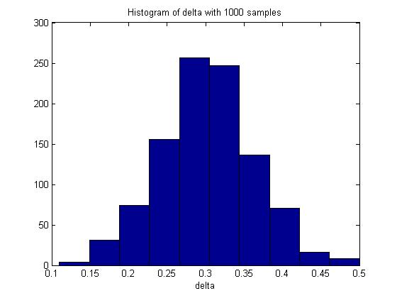
Through Monte Carlo simulation, we can obtain an empirical distribution of delta and carry out inference on the data obtained, such as computing the mean, maximum, variance, standard deviation and the standard error of delta.

Importance Sampling

Motivation

Consider the integral [math]\displaystyle{ \displaystyle I = \int h(x)f(x)\,dx }[/math]

According to basic Monte Carlo Integration, if we can sample from the probability density function [math]\displaystyle{ \displaystyle f(x) }[/math] and feed the samples of [math]\displaystyle{ \displaystyle f(x) }[/math] back to [math]\displaystyle{ \displaystyle h(x) }[/math], [math]\displaystyle{ \displaystyle I }[/math] can be estimated as an average of [math]\displaystyle{ \displaystyle h(x) }[/math] ( i.e. [math]\displaystyle{ \hat{I} = \frac{1}{n} \sum_{i=1}^{n} h(x_i) }[/math] )
However, the Monte Carlo method works when we know how to sample from [math]\displaystyle{ \displaystyle f(x) }[/math]. In the case where it is difficult to sample from [math]\displaystyle{ \displaystyle f(x) }[/math], importance sampling is a technique that we can apply. Importance Sampling relies on another function [math]\displaystyle{ \displaystyle g(x) }[/math] which we know how to sample from.

The above integral can be rewritten as follow:
[math]\displaystyle{ \begin{align} \displaystyle I & = \int h(x)f(x)\,dx \\ & = \int h(x)f(x)\frac{g(x)}{g(x)}\,dx \\ & = \int \frac{h(x)f(x)}{g(x)}g(x)\,dx \\ & = \int y(x)g(x)\,dx \\ & = E_g(y(x)) \\ \end{align} }[/math]
[math]\displaystyle{ where \ y(x) = \frac{h(x)f(x)}{g(x)} }[/math]

The integral can thus be simulated as [math]\displaystyle{ \displaystyle \hat{I} = \frac{1}{n} \sum_{i=1}^{n} Y_i \ , \ where \ Y_i = \frac{h(x_i)f(x_i)}{g(x_i)} }[/math]

Procedure

Suppose we know how to sample from [math]\displaystyle{ \displaystyle g(x) }[/math]

1. Choose a suitable [math]\displaystyle{ \displaystyle g(x) }[/math] and draw n samples [math]\displaystyle{ x_1,x_2....,x_n \sim~ g(x) }[/math]
2. Set [math]\displaystyle{ Y_i =\frac{h(x_i)f(x_i)}{g(x_i)} }[/math]
3. Compute [math]\displaystyle{ \hat{I} = \frac{1}{n}\sum_{i=1}^{n} Y_i }[/math]
   

By the Law of large numbers, [math]\displaystyle{ \displaystyle \hat{I} \rightarrow I }[/math] provided that the sample size n is large enough.

Remarks: One can think of [math]\displaystyle{ \frac{f(x)}{g(x)} }[/math] as a weight to [math]\displaystyle{ \displaystyle h(x) }[/math] in the computation of [math]\displaystyle{ \hat{I} }[/math]

[math]\displaystyle{ \displaystyle i.e. \ \hat{I} = \frac{1}{n}\sum_{i=1}^{n} Y_i = \frac{1}{n}\sum_{i=1}^{n} (\frac{f(x_i)}{g(x_i)})h(x_i) }[/math]

Therefore, [math]\displaystyle{ \displaystyle \hat{I} }[/math] is a weighted average of [math]\displaystyle{ \displaystyle h(x_i) }[/math]

Problem

If [math]\displaystyle{ \displaystyle g(x) }[/math] is not chosen appropriately, then the variance of the estimate [math]\displaystyle{ \hat{I} }[/math] may be very large. Here we actually face a similar problem with Rejection-Acceptance Approach. Consider the second moment of [math]\displaystyle{ \displaystyle I }[/math]:

[math]\displaystyle{ \begin{align} \displaystyle I & = E_g((y(x))^2) \\ & = \int (\frac{h(x)f(x)}{g(x)})^2 g(x) dx \\ & = \int \frac{h^2(x) f^2(x)}{g^2(x)} g(x) dx \\ & = \int \frac{h^2(x)f^2(x)}{g(x)} dx \\ \end{align} }[/math]

When [math]\displaystyle{ \displaystyle g(x) }[/math] is very small, then the above integral could be very large, hence the variance can be very large when g is not chosen appropriately. This occurs when [math]\displaystyle{ \displaystyle g(x) }[/math] has a thinner tail than [math]\displaystyle{ \displaystyle f(x) }[/math] such that the quantity [math]\displaystyle{ \displaystyle \frac{h^2(x)f^2(x)}{g(x)} }[/math] is large.

Remarks:

1. We can actually compute the form of [math]\displaystyle{ \displaystyle g(x) }[/math] to have optimal variance.
Mathematically, it is to find [math]\displaystyle{ \displaystyle g(x) }[/math] subject to [math]\displaystyle{ \displaystyle \min_g [\ E_g([y(x)]^2) - (E_g[y(x)])^2\ ] }[/math]
It can be shown that the optimal [math]\displaystyle{ \displaystyle g(x) }[/math] is [math]\displaystyle{ \displaystyle \frac{|h(x)|f(x)}{\int_{-\infty}^{\infty}|h(s)|f(s)ds} }[/math]. Using the optimal [math]\displaystyle{ \displaystyle g(x) }[/math] will minimize the variance of estimation in Importance Sampling. This is of theoretical interest but not useful in practice. As we can see, if we can actually show the expression of g(x), we must first have the value of the integration---which is what we want in the first place.

2. In practice, we shall choose [math]\displaystyle{ \displaystyle g(x) }[/math] which has similar shape as [math]\displaystyle{ \displaystyle f(x) }[/math] but with a thicker tail than [math]\displaystyle{ \displaystyle f(x) }[/math] in order to avoid the problem mentioned above.

Example

Estimate [math]\displaystyle{ \displaystyle I = Pr(Z\gt 3),\ where\ Z \sim N(0,1) }[/math]

Method 1: Basic Monte Carlo

[math]\displaystyle{ \begin{align} Pr(Z\gt 3) & = \int^\infty_3 f(x)\,dx \\ & = \int^\infty_{-\infty} h(x)f(x)\,dx \end{align} }[/math]
[math]\displaystyle{ where \ h(x) = \begin{cases} 0, & \text{if } x \le 3 \\ 1, & \text{if } x \gt 3 \end{cases} }[/math] [math]\displaystyle{ \ ,\ f(x) = \frac{1}{\sqrt{2\pi}}e^{-\frac{1}{2}x^2} }[/math]

MATLAB code to compute [math]\displaystyle{ \displaystyle I }[/math] from 100 samples of standard normal distribution:

h = randn(100,1) > 3;
I = mean(h)

In one execution of the code, it returns a value of 0 for [math]\displaystyle{ \displaystyle I }[/math], which differs significantly from the true value of [math]\displaystyle{ \displaystyle I \approx 0.0013 }[/math]. The problem of using Basic Monte Carlo in this example is that [math]\displaystyle{ \displaystyle Pr(Z\gt 3) }[/math] has a small value, and hence many points sampled from the standard normal distribution will be wasted. Therefore, although Basic Monte Carlo is a feasible method to compute [math]\displaystyle{ \displaystyle I }[/math], it gives a poor estimation.

Method 2: Importance Sampling

[math]\displaystyle{ \displaystyle I = Pr(Z\gt 3)= \int^\infty_3 f(x)\,dx }[/math]

To apply importance sampling, we have to choose a [math]\displaystyle{ \displaystyle g(x) }[/math] which we will sample from. In this example, we can choose [math]\displaystyle{ \displaystyle g(x) }[/math] to be the probability density function of exponential distribution, normal distribution with mean 0 and variance greater than 1 or normal distribution with mean greater than 0 and variance 1 etc.. For the following, we take [math]\displaystyle{ \displaystyle g(x) }[/math] to be the pdf of [math]\displaystyle{ \displaystyle N(4,1) }[/math].

Procedure:

1. Draw n samples [math]\displaystyle{ x_1,x_2....,x_n \sim~ g(x) }[/math]
2. Calculate [math]\displaystyle{ \begin{align} \frac{f(x)}{g(x)} & = \frac{ \frac{1}{\sqrt{2\pi}}e^{-\frac{1}{2}x^2} }{ \frac{1}{\sqrt{2\pi}}e^{-\frac{1}{2}(x-4)^2} } \\ & = e^{8-4x} \end{align} }[/math]
   
3. Set [math]\displaystyle{ Y_i = h(x_i)e^{8-4x_i}\ with\ h(x) = \begin{cases} 0, & \text{if } x \le 3 \\ 1, & \text{if } x \gt 3 \end{cases} }[/math]
   
4. Compute [math]\displaystyle{ \hat{Y} = \frac{1}{n}\sum_{i=1}^{n} Y_i }[/math]
   

The above procedure from 100 samples of [math]\displaystyle{ \displaystyle g(x) }[/math]can be implemented in MATLAB as follow:

for ii = 1:100
  x = randn + 4 ;
  h = x > 3 ;
  y(ii) = h * exp(8-4*x) ;
end
mean(y)

In one execution of the code, it returns a value of 0.001271 for [math]\displaystyle{ \hat{Y} }[/math], which is much closer to the true value of [math]\displaystyle{ \displaystyle I \approx 0.0013 }[/math]. From many executions of the code, the variance of basic monte carlo is approximately 150 times that of importance sampling. This demonstrates that this method can provide a better estimate than the Basic Monte Carlo method.

Importance Sampling with Normalized Weight and Markov Chain Monte Carlo - October 13th, 2011

Importance Sampling with Normalized Weight

Recall that we can think of [math]\displaystyle{ \displaystyle b(x) = \frac{f(x)}{g(x)} }[/math] as a weight applied to the samples [math]\displaystyle{ \displaystyle h(x) }[/math]. If the form of [math]\displaystyle{ \displaystyle f(x) }[/math] is known only up to a constant, we can use an alternate, normalized form of the weight, [math]\displaystyle{ \displaystyle b^*(x) }[/math]. (This situation arises in Bayesian inference.) Importance sampling with normalized or standard weight is also called indirect importance sampling.

We derive the normalized weight as follows:
[math]\displaystyle{ \begin{align} \displaystyle I & = \int h(x)f(x)\,dx \\ &= \int h(x)\frac{f(x)}{g(x)}g(x)\,dx \\ &= \frac{\int h(x)\frac{f(x)}{g(x)}g(x)\,dx}{\int f(x) dx} \\ &= \frac{\int h(x)\frac{f(x)}{g(x)}g(x)\,dx}{\int \frac{f(x)}{g(x)}g(x) dx} \\ &= \frac{\int h(x)b(x)g(x)\,dx}{\int\ b(x)g(x) dx} \end{align} }[/math]

[math]\displaystyle{ \hat{I}= \frac{\sum_{i=1}^{n} h(x_i)b(x_i)}{\sum_{i=1}^{n} b(x_i)} }[/math]

Then, the normalized weight is [math]\displaystyle{ b^*(x) = \displaystyle \frac{b(x_i)}{\sum_{i=1}^{n} b(x_i)} }[/math]

Markov Chain Monte Carlo

We still want to solve [math]\displaystyle{ I = \displaystyle\int^\ h(x)f(x)\,dx }[/math]

Stochastic Process

A stochastic process [math]\displaystyle{ \{ x_t : t \in T \} }[/math] is a collection of random variables. Variables [math]\displaystyle{ \displaystyle x_t }[/math] take values in some set [math]\displaystyle{ \displaystyle X }[/math] called the space set. The set [math]\displaystyle{ \displaystyle T }[/math] is called the index set.

Markov Chain

A Markov Chain is a stochastic process for which the distribution of [math]\displaystyle{ \displaystyle x_t }[/math] depends only on [math]\displaystyle{ \displaystyle x_{t-1} }[/math]. It is a random process characterized as being memoryless; meaning that the next occurrence of a defined event is only dependent on the current event and not on the sequence of events that preceded it.

  Formal Definition: The process [math]\displaystyle{  \{ x_t : t \in T \} }[/math] is a Markov Chain if [math]\displaystyle{ \displaystyle Pr(x_t|x_0, x_1,..., x_{t-1})= Pr(x_t|x_{t-1}) }[/math] for all [math]\displaystyle{  \{t \in T \} }[/math] and for all [math]\displaystyle{  \{x \in X \} }[/math]

For a Markov Chain, [math]\displaystyle{ \displaystyle f(x_1,...x_n)= f(x_1)f(x_2|x_1)f(x_3|x_2)...f(x_n|x_{n-1}) }[/math]

Real Life Example:
When going for an interview, the employer only looks at your highest education achieved. The employer would not look at the past educations received (elementary school, high school etc.) because the employer believes that the highest education achieved summarizes your previous educations. Therefore, anything before your most recent previous education is irrelevant. In other word, we can say that[math]\displaystyle{ x_t }[/math]is regarded as the summary of [math]\displaystyle{ x_{t-1},...,x_2,x_1 }[/math], so when we need to determine [math]\displaystyle{ x_{t+1} }[/math], we only need to pay attention in [math]\displaystyle{ x_{t} }[/math].

Transition Probabilities

A Transition Probability is the probability of jumping from one state to another state.

  Formal Definition: We call [math]\displaystyle{ \displaystyle P_{ij} = Pr(x_{t+1}=j|x_t=i) }[/math] the transition probability.

That is, P(i,j) is the probability of going to state j from state i. The matrix P whose (i,j) element is [math]\displaystyle{ \displaystyle P_{ij} }[/math] is called the Transition Matrix.

Properties of P:

1) [math]\displaystyle{ \displaystyle P_{ij} \gt = 0 }[/math] The probability of going to another state cannot be negative

2) [math]\displaystyle{ \displaystyle \sum_{\forall i}P_{ij} = 1 }[/math] The probability of going to some state from state i (including remaining in state i) is certainty

Random Walk

Example: Start at one point and flip a coin where [math]\displaystyle{ \displaystyle Pr(H)=p }[/math] and [math]\displaystyle{ \displaystyle Pr(T)=1-p=q }[/math]. Take one step right if heads and one step left if tails. If at an endpoint, stay there. The transition matrix is [math]\displaystyle{ P=\left(\begin{matrix}1&0&0&\dots&\dots&0\\ q&0&p&0&\dots&0\\ 0&q&0&p&\dots&0\\ \vdots&\vdots&\vdots&\ddots&\vdots&\vdots\\ \vdots&\vdots&\vdots&\vdots&\ddots&\vdots\\ 0&0&\dots&\dots&\dots&1 \end{matrix}\right) }[/math]

Let [math]\displaystyle{ \displaystyle P_n }[/math] be the matrix such that its (i,j) element is [math]\displaystyle{ \displaystyle P_{ij}(n) }[/math]. This is called n-step probability.

[math]\displaystyle{ \displaystyle P_n = P^n }[/math]

[math]\displaystyle{ \displaystyle P_1 = P }[/math]

[math]\displaystyle{ \displaystyle P_2 = P^2 }[/math]

Markov Chain Properties and Page Rank - October 18th, 2011

Summary of Terminology

Transition Matrix

A matrix [math]\displaystyle{ \!P }[/math] that defines a Markov Chain has the form:

[math]\displaystyle{ P = \begin{bmatrix} P_{11} & \cdots & P_{1N} \\ \vdots & \ddots & \vdots \\ P_{N1} & \cdots & P_{NN} \end{bmatrix} }[/math]

where [math]\displaystyle{ \!P(i,j) = P_{ij} = Pr(x_{t+1} = j | x_t = i) }[/math], [math]\displaystyle{ \ }[/math] [math]\displaystyle{ \forall t \in [0,T] \!\, }[/math], is the probability of transitioning from state i to state j in the Markov Chain.

n-step Transition matrix

A matrix [math]\displaystyle{ \!P_n }[/math] whose (i,j)^th entry is the probability of moving from state i to state j after n transitions:

[math]\displaystyle{ \!P_n(i,j) = Pr(x_{m+n}=j|x_m = i) }[/math]

If the Markov chain is stationary, then [math]\displaystyle{ \!P_n = P^n }[/math].

Marginal distribution of a Markov Chain

We represent the state at time t as a vector.

[math]\displaystyle{ \mu_t = (\mu_t(1) \; \mu_t(2) \; ... \; \mu_t(n)) }[/math]

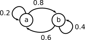
Consider this Markov Chain:

[math]\displaystyle{ \mu_t = (A \; B) }[/math], where A is the probability of being in state a at time t, and B is the probability of being in state b at time t.

For example if [math]\displaystyle{ \mu_t = (0.1 \; 0.9) }[/math], we have a 10% chance of being in state a at time t, and a 90% chance of being in state b at time t.

Suppose we run this Markov chain many times, and record the state at each step.

In this example, we run 4 trials, up until t=5.

t	Trial 1	Trial 2	Trial 3	Trial 4	Observed [math]\displaystyle{ \mu }[/math]
1	a	b	b	a	(0.5, 0.5)
2	b	a	a	a	(0.75, 0.25)
3	a	a	b	a	(0.75, 0.25)
4	b	b	a	b	(0.25, 0.75)
5	b	b	b	a	(0.25, 0.75)

Imagine simulating the chain many times. If we collect all the outcomes at time t from all the chains, the histogram of this data would look like [math]\displaystyle{ \!\mu_t }[/math].

We can find the marginal probabilities as [math]\displaystyle{ \!\mu_n = \mu_0 P^n }[/math]

Stationary Distribution

Let [math]\displaystyle{ \pi = (\pi_i \mid i \in \chi) }[/math] be a vector of non-negative numbers that sum to 1. (i.e. [math]\displaystyle{ \!\pi }[/math] is a pmf)

If [math]\displaystyle{ \!\pi = \pi P }[/math], then [math]\displaystyle{ \!\pi }[/math] is a stationary distribution, also known as an invariant distribution.

Limiting Distribution

A Markov chain has limiting distribution [math]\displaystyle{ \!\pi }[/math] if [math]\displaystyle{ \lim_{n \to \infty} P^n = \begin{bmatrix} \pi \\ \vdots \\ \pi \end{bmatrix} }[/math]

That is, [math]\displaystyle{ \!\pi_j = \lim_{n \to \infty}\left [ P^n \right ]_{ij} }[/math] exists and is independent of i.

Detailed Balance

[math]\displaystyle{ \!\pi }[/math] has the detailed balance property if [math]\displaystyle{ \!\pi_iP_{ij} = P_{ji}\pi_j }[/math]

Theorem

If [math]\displaystyle{ \!\pi }[/math] satisfies detailed balance, then [math]\displaystyle{ \!\pi }[/math] is a stationary distribution.

In other words, if [math]\displaystyle{ \!\pi_iP_{ij} = P_{ji}\pi_j }[/math], then [math]\displaystyle{ \!\pi = \pi P }[/math]

Proof:

[math]\displaystyle{ \!\pi P = \begin{bmatrix}\pi_1 & \pi_2 & \cdots & \pi_N\end{bmatrix} \begin{bmatrix}P_{11} & \cdots & P_{1N} \\ \vdots & \ddots & \vdots \\ P_{N1} & \cdots & P_{NN}\end{bmatrix} }[/math]

Observe that the j^th element of [math]\displaystyle{ \!\pi P }[/math] is

[math]\displaystyle{ \!\left [ \pi P \right ]_j = \pi_1 P_{1j} + \pi_2 P_{2j} + \dots + \pi_N P_{Nj} }[/math]

[math]\displaystyle{ \! = \sum_{i=1}^N \pi_i P_{ij} }[/math]

[math]\displaystyle{ \! = \sum_{i=1}^N P_{ji} \pi_j }[/math], by the definition of detailed balance.

[math]\displaystyle{ \! = \pi_j \sum_{i=1}^N P_{ji} }[/math]

[math]\displaystyle{ \! = \pi_j }[/math], as the sum of the entries in a column of P must sum to 1.

So [math]\displaystyle{ \!\pi = \pi P }[/math].

Example

Find the marginal distribution of

Start by generating the matrix P.

[math]\displaystyle{ \!P = \begin{pmatrix} 0.2 & 0.8 \\ 0.6 & 0.4 \end{pmatrix} }[/math]

We must assume some starting value for [math]\displaystyle{ \mu_0 }[/math]

[math]\displaystyle{ \!\mu_0 = \begin{pmatrix} 0.1 & 0.9 \end{pmatrix} }[/math]

For t = 1, the marginal distribution is

[math]\displaystyle{ \!\mu_1 = \mu_0 P }[/math]

Notice that this [math]\displaystyle{ \mu }[/math] converges.

If you repeatedly run:

[math]\displaystyle{ \!\mu_{i+1} = \mu_i P }[/math]

It converges to [math]\displaystyle{ \mu = \begin{pmatrix} 0.4286 & 0.5714 \end{pmatrix} }[/math]

This can be seen by running the following Matlab code:

P = [0.2 0.8; 0.6 0.4];
mu = [0.1 0.9];           
while 1                   
  mu_old = mu;         
  mu = mu * P;
  if mu_old == mu      
    disp(mu);
    break;
  end
end

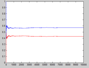
Another way of looking at this simple question is that we can see whether the ultimate pmf converges:

Let [math]\displaystyle{ \hat{p_n}(1)=\frac{1}{n}\sum_{k=1}^n I(X_k=1) }[/math] denote the estimator of the stationary probability of state 1,[math]\displaystyle{ \hat{p_n}(2)=\frac{1}{n}\sum_{k=1}^n I(X_k=2) }[/math] denote the estimator of the stationary probability of state 2, where [math]\displaystyle{ \displaystyle I(X_k=1) }[/math] and [math]\displaystyle{ \displaystyle I(X_k=2) }[/math] are indicator variables which equal 1 if [math]\displaystyle{ X_k=1 }[/math](or [math]\displaystyle{ X_k=2 }[/math] for the latter one).

Matlab codes for this explanation is

n=1;
if rand<0.1
    x(1)=1;
else
    x(1)=0;
end
p1(1)=sum(x)/n;
p2(1)=1-p1(1);
for i=2:10000
    n=n+1;
    if (x(i-1)==1&rand<0.2)|(x(i-1)==0&rand<0.6)
        x(i)=1;
    else
        x(i)=0;
    end
    p1(i)=sum(x)/n;
    p2(i)=1-p1(i);   
end
plot(p1,'red');
hold on;
plot(p2)

The results can be easily seen from the graph below:

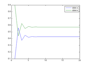
Additionally, we can plot the marginal distribution as it converges without estimating it. The following Matlab code shows this:

%transition matrix
P=[0.2 0.8; 0.6 0.4];
%mu at time 0
mu=[0.1 0.9];
%number of points for simulation
n=20;
for i=1:n
    mu_a(i)=mu(1);
    mu_b(i)=mu(2);
    mu=mu*P;
end
t=[1:n];
plot(t, mu_a, t, mu_b);
hleg1=legend('state a', 'state b');

Note that there are chains with stationary distributions that don't converge (the chain might not naturally reach the stationary distribution, and isn't limiting). An example of this is:

[math]\displaystyle{ P = \begin{pmatrix} 0 & 1 & 0 \\ 0 & 0 & 1 \\ 1 & 0 & 0 \end{pmatrix}, \mu_0 = \begin{pmatrix} 1/3 & 1/3 & 1/3 \end{pmatrix} }[/math]

[math]\displaystyle{ \!\mu_0 }[/math] is a stationary distribution, so [math]\displaystyle{ \!\mu P }[/math] is the same for all iterations.

But,

[math]\displaystyle{ P^{1000} = \begin{pmatrix} 0 & 0 & 1 \\ 1 & 0 & 0 \\ 0 & 1 & 0 \end{pmatrix} \ne \begin{pmatrix} \mu \\ \mu \\ \mu \end{pmatrix} }[/math]

So [math]\displaystyle{ \!\mu }[/math] is not a limiting distribution. Also, if

[math]\displaystyle{ \mu = \begin{pmatrix} 0.2 & 0.1 & 0.7 \end{pmatrix} }[/math]

Then [math]\displaystyle{ \!\mu = \mu P }[/math] does not converge.

This can be observed through the following Matlab code.

P = [0 0 1; 1 0 0; 0 1 0];
mu = [0.2 0.1 0.7];       
for i= 1:4                
  mu = mu * P;
  disp(mu);
end

This outputs

0.1000    0.7000    0.2000
0.7000    0.2000    0.1000
0.2000    0.1000    0.7000
0.1000    0.7000    0.2000

Note that [math]\displaystyle{ \!\mu_1 = \!\mu_4 }[/math], which indicates that [math]\displaystyle{ \!\mu }[/math] will cycle forever.

This means that this chain has a stationary distribution, but is not limiting.

Page Rank

Page Rank was the original ranking algorithm used by Google's search engine to rank web pages.<ref> http://ilpubs.stanford.edu:8090/422/ </ref> The algorithm was created by the founders of Google, Larry Page and Sergey Brin as part of Page's PhD thesis. When a query is entered in a search engine, there are a set of web pages which are matched by this query, but this set of pages must be ordered by their "importance" in order to identify the most meaningful results first. Page Rank is an algorithm which assigns importance to every web page based on the links in each page.

Intuition

We can represent web pages by a set of nodes, where web links are represented as edges connecting these nodes. Based on our intuition, there are three main factors in deciding whether a web page is important or not.

1. A web page is important if many other pages point to it.
2. The more important a webpage is, the more weight is placed on its links.
3. The more links a webpage has, the less weight is placed on its links.

Modelling

We can model the set of links as a N-by-N matrix L, where N is the number of web pages we are interested in:

[math]\displaystyle{ L_{ij} = \left\{ \begin{array}{lr} 1 : \text{if page j points to i}\\ 0 : \text{otherwise} \end{array} \right. }[/math]

The number of outgoing links from page j is

[math]\displaystyle{ c_j = \sum_{i=1}^N L_{ij} }[/math]

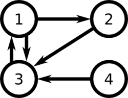
For example, consider the following set of links between web pages:

According to the factors relating to importance of links, we can consider two possible rankings :

[math]\displaystyle{ \displaystyle 3 \gt 2 \gt 1 \gt 4 }[/math]

or

[math]\displaystyle{ \displaystyle 3\gt 1\gt 2\gt 4 }[/math] if we consider that the high importance of the link from 3 to 1 is more influent than the fact that there are two outgoing links from page 1 and only one from page 2.

We have [math]\displaystyle{ L = \begin{bmatrix} 0 & 0 & 1 & 0 \\ 1 & 0 & 0 & 0 \\ 1 & 1 & 0 & 1 \\ 0 & 0 & 0 & 0 \end{bmatrix} }[/math], and [math]\displaystyle{ c = \begin{pmatrix}2 & 1 & 1 & 1\end{pmatrix} }[/math]

We can represent the ranks of web pages as the vector P, where the i^th element is the rank of page i:

[math]\displaystyle{ P_i = (1-d) + d\sum_j \frac{L_{ij}}{c_j} P_j }[/math]

Here we take the sum of the weights of the incoming links, where links are reduced in weight if the linking page has a lot of outgoing links, and links are increased in weight if the linking page has a lot of incoming links.

We don't want to completely ignore pages with no incoming links, which is why we add the constant (1 - d).

If

[math]\displaystyle{ L = \begin{bmatrix} L_{11} & \cdots & L_{1N} \\ \vdots & \ddots & \vdots \\ L_{N1} & \cdots & L_{NN} \end{bmatrix} }[/math]

[math]\displaystyle{ D = \begin{bmatrix} c_1 & \cdots & 0 \\ \vdots & \ddots & \vdots \\ 0 & \cdots & c_N \end{bmatrix} }[/math]

Then [math]\displaystyle{ D^{-1} = \begin{bmatrix} c_1^{-1} & \cdots & 0 \\ \vdots & \ddots & \vdots \\ 0 & \cdots & c_N^{-1} \end{bmatrix} }[/math]

[math]\displaystyle{ \!P = (1-d)e + dLD^{-1}P }[/math]

where [math]\displaystyle{ \!e = \begin{pmatrix} 1 \\ \vdots \\ 1 \end{pmatrix} }[/math] is the vector with all 1's

To simplify the problem, we let [math]\displaystyle{ \!e^T P = N \Rightarrow \frac{e^T P}{N} = 1 }[/math]. This means that the average importance of all pages on the internet is 1.

Then [math]\displaystyle{ \!P = (1-d)\frac{ee^TP}{N} + dLD^{-1}P }[/math]

[math]\displaystyle{ \! = \left [ (1-d)\frac{ee^T}{N} + dLD^{-1} \right ] P }[/math]

[math]\displaystyle{ \! = \left [ \left ( \frac{1-d}{N} \right ) E + dLD^{-1} \right ] P }[/math], where [math]\displaystyle{ E }[/math] is an NxN matrix filled with ones.

Let [math]\displaystyle{ \!A = \left [ \left ( \frac{1-d}{N} \right ) E + dLD^{-1} \right ] }[/math]

Then [math]\displaystyle{ \!P = AP }[/math].

Note that P is a stationary distribution and, more importantly, P is an eigenvector of A with eigenvalue 1. Therefore, we can find the ranks of all web pages by solving this equation for P.

We can find the vector P for the example above, using the following Matlab code:

L = [0 0 1 0; 1 0 0 0; 1 1 0 1; 0 0 0 0];
D = [2 0 0 0; 0 1 0 0; 0 0 1 0; 0 0 0 1];
d = 0.8 ;% pages with no links get a weight of 0.2
N = 4 ;

A = ((1-d)/N) * ones(N) + d * L * inv(D);
[EigenVectors, EigenValues] = eigs(A)
s=sum(EigenVectors(:,1));% we should note that the average entry of P should be 1 according to our assumption
P=(EigenVectors(:,1))/s*N

This outputs:

EigenVectors =
 -0.6363             0.7071             0.7071            -0.0000          
 -0.3421            -0.3536 + 0.3536i  -0.3536 - 0.3536i  -0.7071          
 -0.6859            -0.3536 - 0.3536i  -0.3536 + 0.3536i   0.0000          
 -0.0876             0.0000 + 0.0000i   0.0000 - 0.0000i   0.7071          

EigenValues =
  1.0000                  0                  0                  0          
       0            -0.4000 - 0.4000i        0                  0          
       0                  0            -0.4000 + 0.4000i        0          
       0                  0                  0             0.0000       

P =

   1.4528
   0.7811
   1.5660
   0.2000

Note that there is an eigenvector with eigenvalue 1. The reason why there always exist a 1-eigenvector is that A is a stochastic matrix.

Thus our vector P is [math]\displaystyle{ \begin{bmatrix}1.4528 \\ 0.7811 \\ 1.5660\\ 0.2000 \end{bmatrix} }[/math]

However, this method is not practical, because there are simply too many web pages on the internet. So instead Google uses a method to approximate an eigenvector with eigenvalue 1.

Note that page three has the rank with highest magnitude and page four has the rank with lowest magnitude, as expected.

Markov Chain Monte Carlo - Metropolis-Hastings - October 25th, 2011

We want to find [math]\displaystyle{ \int h(x)f(x)\, \mathrm dx }[/math], but we don't know how to sample from [math]\displaystyle{ \,f }[/math].

We have seen simple techniques before. This one is used in real life. It consists of the search of a Markov Chain such that its stationary distribution is [math]\displaystyle{ \,f }[/math].

Main procedure

Let us suppose that [math]\displaystyle{ \,q(y|x) }[/math] is a friendly distribution: we can sample from this function.

1/ Initialize the chain with [math]\displaystyle{ \,x_{i} }[/math] and set [math]\displaystyle{ \,i=0 }[/math].

2/ Draw a point from [math]\displaystyle{ \,q(y|x) }[/math] i.e. [math]\displaystyle{ \,Y \backsim q(y|x_{i}) }[/math].

3/ Evaluate [math]\displaystyle{ \,r(x,y)=min\left\{\frac{f(y)}{f(x)}\frac{q(x|y)}{q(y|x)},1\right\} }[/math]

4/ Draw a point [math]\displaystyle{ \,U \backsim Unif[0,1] }[/math].

5/ [math]\displaystyle{ \,x_{i+1}=\begin{cases}y & \text{ if } U\lt r \\x_{i} & \text{ otherwise } \end{cases} }[/math].

6/[math]\displaystyle{ \,i=i+1 }[/math]. Go back to 2/.

Remark 1

A very common choice for [math]\displaystyle{ \,q(y|x) }[/math] is [math]\displaystyle{ \,N(y;x,b^{2}) }[/math], a normal distribution centered at the current point.

Note : In this case [math]\displaystyle{ \,q(y|x) }[/math] is symmetric i.e. [math]\displaystyle{ \,q(y|x)=q(x|y) }[/math].

(Because [math]\displaystyle{ \,q(y|x)=\frac{1}{\sqrt{2\pi}b}e^{-\frac{1}{2b^{2}}(y-x)^{2}} }[/math] and [math]\displaystyle{ \,(y-x)^{2}=(x-y)^{2} }[/math]).

Thus we have [math]\displaystyle{ \,\frac{q(x|y)}{q(y|x)}=1 }[/math], which implies :

[math]\displaystyle{ \,r(x,y)=min\left\{\frac{f(y)}{f(x)},1\right\} }[/math].

In general, if [math]\displaystyle{ \,q(x|y) }[/math] is symmetric then the algorithm is called Metropolis in reference to the original algorithm (made in 1953)<ref>http://en.wikipedia.org/wiki/Equations_of_State_Calculations_by_Fast_Computing_Machines</ref>.

Remark 2

The value y is accepted if [math]\displaystyle{ \,u\lt min\left\{\frac{f(y)}{f(x)},1\right\} }[/math] so it is accepted with the probability [math]\displaystyle{ \,min\left\{\frac{f(y)}{f(x)},1\right\} }[/math].

Thus, if [math]\displaystyle{ \,f(y)\gt f(x) }[/math], then [math]\displaystyle{ \,y }[/math] is always accepted.

In fact the value of the pdf is high around a point [math]\displaystyle{ \,y_(1) }[/math] the pdf is, the more the random variable takes value around this point, so we want a high probability of acceptance.

Example

[math]\displaystyle{ \,f(x)=\frac{1}{\pi^{2}}\frac{1}{1+x^{2}} }[/math]

Then, we have [math]\displaystyle{ \,f(x)\propto\frac{1}{1+x^{2}} }[/math].

And let us take [math]\displaystyle{ \,q(x|y)=\frac{1}{\sqrt{2\pi}b}e^{-\frac{1}{2b^{2}}(y-x)^{2}} }[/math].

Then [math]\displaystyle{ \,q(x|y) }[/math] is symmetric.

Therefore Y can be simplified.

We get :

[math]\displaystyle{ \,\begin{align} \displaystyle r(x,y) & =min\left\{\frac{f(y)}{f(x)}\frac{q(x|y)}{q(y|x)},1\right\} \\ & =min\left\{\frac{f(y)}{f(x)},1\right\} \\ & =min\left\{ \frac{ \frac{1}{1+y^{2}} }{ \frac{1}{1+x^{2}} },1\right\}\\ & =min\left\{ \frac{1+x^{2}}{1+y^{2}},1\right\}\\ \end{align} }[/math].

The Matlab code of the algorithm is the following :

clear all
close all
clc
b=2;
x(1)=randn;
for i=2:10000
    y=b*randn+x(i-1);
    r=min((1+x(i-1)^2)/(1+y^2),1);
    u=rand;
    if u<r
        x(i)=y;
    else
        x(i)=x(i-1);
    end
    
end
hist(x(5000:end));
%We don't display the 5000 first points because they
%don't show the limiting behaviour of the Markov Chain

As we can see, the choice of the value of b is made by us.

Changing this value has a significant impact on the results we obtain.

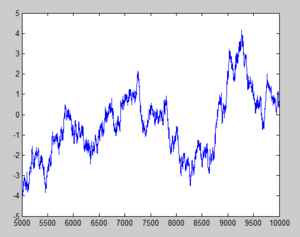
Example with [math]\displaystyle{ \,b=0.1 }[/math] (Also with graph after we run j=5000:10000; plot(j,x(5000:10000)):

File:redaccoursb01.JPG

With [math]\displaystyle{ \,b=0.1 }[/math], the chain takes small steps so the chain doesn't explore enough of the sample space. It doesn't give an accurate report of the function we want to sample.

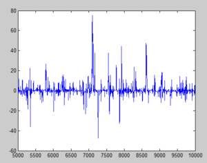
Example with [math]\displaystyle{ \,b=10 }[/math] :

File:redaccoursb10.JPG

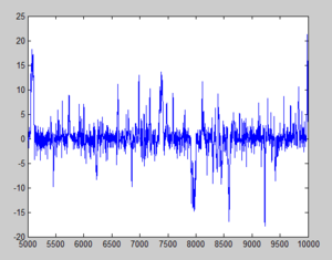
With [math]\displaystyle{ \,b=10 }[/math], jumps are very unlikely to be accepted as they deviate far from the mean (i.e. [math]\displaystyle{ \,y }[/math] is rejected as [math]\displaystyle{ \ u\lt r }[/math] and [math]\displaystyle{ \,x(i)=x(i-1) }[/math] most of the time, hence most sample points stay fairly close to the origin. The third graph that resembles white noise (as in the case of [math]\displaystyle{ \,b=2 }[/math]) indicates better sampling as more points are covered and accepted. For [math]\displaystyle{ \,b=0.1 }[/math], we have lots of jumps but most values are not repeated, hence the stationary distribution is less obvious; whereas in the [math]\displaystyle{ \,b=10 }[/math] case, many points remains around 0. Approximately 73% were selected as x(i-1).

Example with [math]\displaystyle{ \,b=2 }[/math] :

File:redaccoursb2.JPG

With [math]\displaystyle{ \,b=2 }[/math], we get a more accurate result as we avoid these extremes. Approximately 37% were selected as x(i-1).

If the sample from the Markov Chain starts to look like the target distribution quickly, we say the chain is mixing well.

Theory and Applications of Metropolis-Hastings - October 27th, 2011

As mentioned in the previous section, the idea of the Metropolis-Hastings (MH) algorithm is to produce a Markov chain that converges to a stationary distribution [math]\displaystyle{ f }[/math] which we are interested in sampling from.

Convergence

One important fact to check is that [math]\displaystyle{ \displaystyle f }[/math] is indeed a stationary distribution in the MH scheme. For this, we can appeal to the implications of the detailed balance property:

Given a probability vector [math]\displaystyle{ \!\pi }[/math] and a transition matrix [math]\displaystyle{ \displaystyle P }[/math], [math]\displaystyle{ \!\pi }[/math] has the detailed balance property if [math]\displaystyle{ \!\pi_iP_{ij} = P_{ji}\pi_j }[/math]

If [math]\displaystyle{ \!\pi }[/math] satisfies detailed balance, then it is a stationary distribution.

The above definition applies to the case where the states are discrete. In the continuous case, [math]\displaystyle{ \displaystyle f }[/math] satisfies detailed balance if [math]\displaystyle{ \displaystyle f(x)p(x,y)=f(y)p(y,x) }[/math]. Where [math]\displaystyle{ \displaystyle p(x,y) }[/math] and [math]\displaystyle{ \displaystyle p(y,x) }[/math] are the probabilities of transitioning from x to y and y to x respectively. If we can show that [math]\displaystyle{ \displaystyle f }[/math] has the detailed balance property, we can conclude that it is a stationary distribution. Because [math]\displaystyle{ \int^{}_y f(y)p(y,x)dy=\int^{}_y f(x)p(x,y)dy=f(x) }[/math].

In the MH algorithm, we use a proposal distribution to generate y~[math]\displaystyle{ \displaystyle q(y|x) }[/math], and accept y with probability [math]\displaystyle{ min\left\{\frac{f(y)}{f(x)}\frac{q(x|y)}{q(y|x)},1\right\} }[/math]

Suppose, without loss of generality, that [math]\displaystyle{ \frac{f(y)}{f(x)}\frac{q(x|y)}{q(y|x)}\lt 1 }[/math]

[math]\displaystyle{ \,P(x,y) }[/math]:

1. if the proposal distribution generate y
2. we accept y

[math]\displaystyle{ \,P(y,x) }[/math]:

1. if the proposal distribution generate x
2. we accept x

[math]\displaystyle{ \,r(x,y) = \frac{f(x)}{f(y)} \frac{q(x|y)}{q(y|x)} }[/math]

[math]\displaystyle{ \,r(y,x) = 1 }[/math]

[math]\displaystyle{ \,P(x,y) = q(y|x)r(x,y) = q(y|x) \frac{f(y)}{f(x)} \frac{q(x|y)}{q(y|x)} = \frac{f(y)q(x|y)}{f(x)} }[/math]

[math]\displaystyle{ \,f(x)P(x,y) = f(y)q(x|y) }[/math]

[math]\displaystyle{ \,P(y,x) = q(x|y)r(y,x) = q(x|y) }[/math]

[math]\displaystyle{ \,f(x)P(x,y) = f(y)P(y,x) }[/math]

Thus, detailed balance holds.

i.e. [math]\displaystyle{ \,f(x) }[/math] is stationary distribution

It can be shown (although not here) that [math]\displaystyle{ f }[/math] is a limiting distribution as well. Therefore, the MH algorithm generates a sequence whose distribution converges to [math]\displaystyle{ f }[/math], the target.

Implementation

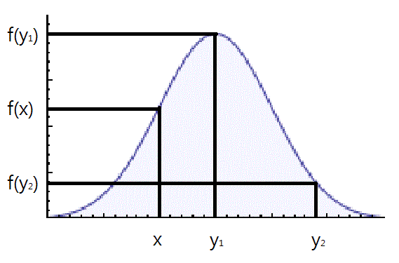
In the implementation of MH, the proposal distribution is commonly chosen to be symmetric, which simplifies the calculations as well as rendering the algorithm more intuitively understandable. The MH algorithm can usually be regarded as a random walk along the distribution we want to sample from. Suppose we have a distribution [math]\displaystyle{ f }[/math]:

Suppose we start the walk at point [math]\displaystyle{ x }[/math]. The point [math]\displaystyle{ y_{1} }[/math] is in a denser region than [math]\displaystyle{ x }[/math], therefore, the walk will always progress from [math]\displaystyle{ x }[/math] to [math]\displaystyle{ y_{1} }[/math]. On the other hand, [math]\displaystyle{ y_{2} }[/math] is in a less dense region, so it is not certain that the walk will progress from [math]\displaystyle{ x }[/math] to [math]\displaystyle{ y_{2} }[/math]. From the perspective of the MH algorithm:

[math]\displaystyle{ r(x,y_{1})=min(\frac{f(y_{1})}{f(x)},1)=1 }[/math] since [math]\displaystyle{ f(y_{1})\gt f(x) }[/math]. Values with higher densities will always be accepted if generated.

[math]\displaystyle{ r(x,y_{2})=\frac{f(y_{2})}{f(x)} }[/math]. The lower the density of [math]\displaystyle{ y_{2} }[/math] is, the less chance it will have of being accepted.

A certain class of proposal distributions can be written in the form:

[math]\displaystyle{ \,y|x_i = x_i + \epsilon_i }[/math]

where [math]\displaystyle{ \,\epsilon_i = g(|x-y|) }[/math]

The density depends only on the distance between the current point and the next one (which can be seen as the "step" being taken). These proposal distributions give the Markov chain the random walk nature. The normal distribution that we frequently use in our examples satisfies the above definition.

In actual implementations of the MH algorithm, the proposal distribution needs to be chosen judiciously, because not all proposals will work well with all target distributions we want to sample from. Take a trimodal distribution for example:

File:trimodal.jpg

If we choose the proposal distribution to be a standard normal as we have done before, problems will arise. The low densities between the peaks means that the MH algorithm will almost never walk to any points generated in these regions and get stuck at one peak. One way to address this issue is to increase the variance, so that the steps will be large enough to cross the gaps. Of course, in this case, it would probably be beneficial to come up with a different proposal function. As a rule of thumb, such functions should result in an approximately 50% acceptance rate for generated points.

Simulated Annealing

Metropolis-Hastings is very useful in simulation solutions to optimization problems. One such application is simulated annealing, which addresses the problems of minimizing a function [math]\displaystyle{ h(x) }[/math]. This method will not always produce the global solution, but it is intuitively simple and easy to implement.

Consider [math]\displaystyle{ e^{\frac{-h(x)}{T}} }[/math], maximizing this expression is equivalent to minimizing [math]\displaystyle{ h(x) }[/math]. Suppose [math]\displaystyle{ \mu }[/math] is the maximizing value, then construct a gaussian distribution [math]\displaystyle{ e^{-\frac{(x-\mu)^2}{T}} }[/math]. When many samples are taken from this distribution, the mean will converge to the desired maximizing value. The annealing comes into play by lowering T (the temperature) as the sampling progresses, making the distribution narrower. The steps of simulated annealing are outlined below:

1. start with a random [math]\displaystyle{ x }[/math] and set T to a large number

2. generate [math]\displaystyle{ y }[/math] from a proposal distribution [math]\displaystyle{ q(y|x) }[/math], which should be symmetric

3. accept [math]\displaystyle{ y }[/math] with probability [math]\displaystyle{ min(\frac{f(y)}{f(x)},1) }[/math]

4. decrease T, and then go to step 2

References

<references/>

Simulated Annealing and Gibbs Sampling - November 1, 2011

continued from previous lecture...

We will now look at a couple cases where [math]\displaystyle{ \displaystyle h(y) \gt h(x) }[/math] or [math]\displaystyle{ \displaystyle h(y) \lt h(x) }[/math], and explore whether to accept or reject [math]\displaystyle{ y }[/math].

Recall r(x,y)=min{[math]\displaystyle{ \frac{f(y)}{f(x)} }[/math],1} where [math]\displaystyle{ \frac{f(y)}{f(x)} = \frac{e^{\frac{-h(x)}{T}}}{e^{\frac{-h(y)}{T}}} = e^{\frac{h(x)-h(y)}{T}} }[/math]. And r(x,y) represents the probability of accepting [math]\displaystyle{ y }[/math].

Cases

Case a) Suppose [math]\displaystyle{ \displaystyle h(y) \lt h(x) }[/math]. Since we want to find the minimum value for [math]\displaystyle{ \displaystyle h(x) }[/math], and the point [math]\displaystyle{ \displaystyle y }[/math] creates a lower value than our previous point, we accept the new point. Mathematically, [math]\displaystyle{ \displaystyle h(y) \lt h(x) }[/math] implies that:

[math]\displaystyle{ \frac{f(y)}{f(x)} \gt 1 }[/math]. Therefore, [math]\displaystyle{ \displaystyle r = 1 }[/math]. So, we will always accept [math]\displaystyle{ \displaystyle y }[/math].

Case b) Suppose [math]\displaystyle{ \displaystyle h(y) \gt h(x) }[/math]. This is bad, since our goal is to minimize [math]\displaystyle{ \displaystyle h(x) }[/math]. However, we may still accept [math]\displaystyle{ \displaystyle y }[/math] with a some chance:

[math]\displaystyle{ \frac{f(y)}{f(x)} \lt 1 }[/math]. Therefore, [math]\displaystyle{ \displaystyle r \lt 1 }[/math]. So, we may accept [math]\displaystyle{ \displaystyle y }[/math] with probability [math]\displaystyle{ \displaystyle r }[/math].

Next, we will look at these cases as [math]\displaystyle{ \displaystyle T\to0 }[/math].

As [math]\displaystyle{ \displaystyle T\to0 }[/math] and case a) happens, [math]\displaystyle{ e^{\frac{h(x)-h(y)}{T}} }[/math] approaches infinity, so we will always accept [math]\displaystyle{ \displaystyle y }[/math].

As [math]\displaystyle{ \displaystyle T\to0 }[/math] and case b) happens, [math]\displaystyle{ e^{\frac{h(x)-h(y)}{T}} }[/math] approaches zero, so the probability that [math]\displaystyle{ \displaystyle y }[/math] will be accepted gets extremely small.

It is worth noting that if we simply start with a small value of T, we may end up rejecting all the generated points, and hence we will get stuck somewhere in the function (due to case b)). It is therefore necessary to start with a large value of T in order to explore the whole function.

Example

Let [math]\displaystyle{ \displaystyle h(x) = (x-2)^2 }[/math]. The graph of it is:

500

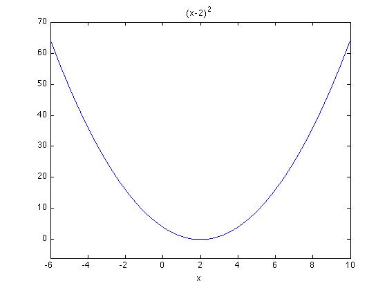
Then, [math]\displaystyle{ e^{\frac{-h(x)}{T}} = e^{\frac{-(x-2)^2}{T}} }[/math] . Take an initial value of T = 20. A graph of this is:

500

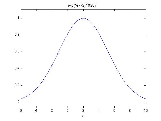
In comparison, we look a graph of T = 0.2:

500

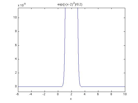
One can see that with a low T value, the graph has a lot of r = 0, and r >1, while having a bigger T value gives smoother transitions in the graph.

The MATLAB code for the above graphs are:

ezplot('(x-2)^2',[-6,10])
ezplot('exp((-(x-2)^2)/20)',[-6,10])
ezplot('exp((-(x-2)^2)/0.2)',[-6,10])

Gibbs Sampling

Gibbs sampling is another Markov chain Monte Carlo method, similar to Metropolis-Hastings. There are two main differences between Metropolis-Hastings and Gibbs sampling. First, the candidate state is always accepted as the next state in Gibbs sampling. Second, it is assumed that the full conditional distributions are known, i.e. [math]\displaystyle{ P(X_i=x|X_j=x_j, \forall j\neq i) }[/math] for all [math]\displaystyle{ \displaystyle i }[/math].

For example, if we want to sample from [math]\displaystyle{ \, f_{X,Y}(x,y) }[/math], we need to know how to sample from [math]\displaystyle{ \, f_{X|Y}(x|y) }[/math] and [math]\displaystyle{ \, f_{Y|X}(y|x) }[/math]. Suppose the chain starts with [math]\displaystyle{ \,(X_0,Y_0) }[/math] and [math]\displaystyle{ (X_1,Y_1), \dots , (X_n,Y_n) }[/math] have been sampled. Then,

[math]\displaystyle{ \, (X_{n+1},Y_{n+1})=(f_{X|Y}(x|Y_n),f_{Y|X}(y|X_n)) }[/math]

Gibbs sampling turns a multi-dimensional distribution into a set of one-dimensional distributions. If we want to sample from

[math]\displaystyle{ P_{X^1,\dots ,X^p}(x^1,\dots ,x^p) }[/math]

and the full conditionals are known, then:

[math]\displaystyle{ X^1_{n+1}=f(X^1|X^2_n,\dots ,X^p_n) }[/math]

[math]\displaystyle{ \vdots }[/math]

[math]\displaystyle{ X^p_{n+1}=f(X^p|X^1_n,\dots ,X^{p-1}_n) }[/math]

With Gibbs sampling, we can simulate [math]\displaystyle{ \displaystyle n }[/math] random variables sequentially from [math]\displaystyle{ \displaystyle n }[/math] univariate conditionals rather than generating one [math]\displaystyle{ n }[/math]-dimensional vector using the full joint distribution, which could be a lot more complicated.

Computational inference deals with probabilistic graphical models. Gibbs sampling is useful here: graphical models show the dependence relations among random variables. For instance, Bayesian networks are graphical models represented using directed acyclic graphs. Looking at such a graphical model tells us on which random variable the distribution of a certain random variable depends (i.e. its parent). The model can be used to "factor" a joint distribution into conditional distributions.

File:stat341 nov 1 graphical model.png

Sample graphical model of five RVs

For example, consider the five random variables A, B, C, D, and E. Without making any assumptions about dependence relations among them, all we know is

[math]\displaystyle{ \, P(A,B,C,D,E)= }[/math][math]\displaystyle{ \, P(A|B,C,D,E) P(B|C,D,E) P(C|D,E) P(D|E) P(E) }[/math]

However, if we know the relation between the random variables, e.g. given the graphical model on the left, we can simplify this expression:

[math]\displaystyle{ \, P(A,B,C,D,E)=P(A) P(B|A) P(C|A) P(D|C) P(E|C) }[/math]

Although the joint distribution may be very complicated, the conditional distributions may not be.

Check out the following notes on Gibbs sampling:

• MCMC and Gibbs Sampling, MIT Lecture Notes
• chapter 7.4 in Notes on Computational Methods in Statistics
• chapter 4.9 in Introduction to Probability Models by Sheldon Ross

Example of Gibbs sampling: Multi-variate normal

We'd like to generate samples from a bivariate normal with parameters

[math]\displaystyle{ \mu = \begin{bmatrix}1\\ 2 \end{bmatrix} = \begin{bmatrix}\mu_1 \\ \mu_2 \end{bmatrix} }[/math] and [math]\displaystyle{ \sigma = \begin{bmatrix}1 && 0.9 \\ 0.9 && 1 \end{bmatrix}= \begin{bmatrix}1 && \rho \\ \rho && 1 \end{bmatrix} }[/math]

The conditional distributions of multi-variate normal random variables are also normal:

[math]\displaystyle{ \, f(x_1|x_2)=N(\mu_1 + \rho(x_2-\mu_2), 1-\rho^2) }[/math]

[math]\displaystyle{ \, f(x_2|x_1)=N(\mu_2 + \rho(x_1-\mu_1), 1-\rho^2) }[/math]

(In general, if the joint distribution has parameters

[math]\displaystyle{ \mu = \begin{bmatrix}\mu_1 \\ \mu_2 \end{bmatrix} }[/math] and [math]\displaystyle{ \Sigma = \begin{bmatrix} \Sigma _{1,1} && \Sigma _{1,2} \\ \Sigma _{2,1} && \Sigma _{2,2} \end{bmatrix} }[/math]

then the conditional distribution [math]\displaystyle{ \, f(x_1|x_2) }[/math] has mean [math]\displaystyle{ \, \mu_1 + \Sigma _{1,2}(\Sigma _{1,1})^{-1}(x_2-\mu_2) }[/math] and variance [math]\displaystyle{ \, \Sigma _{1,1}-\Sigma _{1,2}(\Sigma _{2,2})^{-1}\Sigma _{2,1}) }[/math].

To be continued...