stat946f11
Editor Sign Up
Sign up for your presentation
Assignments
Introduction
Motivation
Graphical probabilistic models provide a concise representation of various probabilistic distributions that are found in many real world applications. Some interesting areas include medical diagnosis, computer vision, language, analyzing gene expression data, etc. A problem related to medical diagnosis is, "detecting and quantifying the causes of a disease". This question can be addressed through the graphical representation of relationships between various random variables (both observed and hidden). This is an efficient way of representing a joint probability distribution.
Graphical models are excellent tools to burden the computational load of probabilistic models. Suppose we want to model a binary image. If we have 256 by 256 image then our distribution function has [math]\displaystyle{ 2^{256*256}=2^{65536} }[/math] outcomes. Even very simple tasks such as marginalization of such a probability distribution over some variables can be computationally intractable and the load grows exponentially versus number of the variables. In practice and in real world applications we generally have some kind of dependency or relation between the variables. Using such information, can help us to simplify the calculations. For example for the same problem if all the image pixels can be assumed to be independent, marginalization can be done easily. One of the good tools to depict such relations are graphs. Using some rules we can indicate a probability distribution uniquely by a graph, and then it will be easier to study the graph instead of the probability distribution function (PDF). We can take advantage of graph theory tools to design some algorithms. Though it may seem simple but this approach will simplify the commutations and as mentioned help us to solve a lot of problems in different research areas.
Notation
We will begin with short section about the notation used in these notes. Capital letters will be used to denote random variables and lower case letters denote observations for those random variables:
- [math]\displaystyle{ \{X_1,\ X_2,\ \dots,\ X_n\} }[/math] random variables
- [math]\displaystyle{ \{x_1,\ x_2,\ \dots,\ x_n\} }[/math] observations of the random variables
The joint probability mass function can be written as:
or as shorthand, we can write this as [math]\displaystyle{ p( x_1, x_2, \dots, x_n ) }[/math]. In these notes both types of notation will be used. We can also define a set of random variables [math]\displaystyle{ X_Q }[/math] where [math]\displaystyle{ Q }[/math] represents a set of subscripts.
Example
Let [math]\displaystyle{ A = \{1,4\} }[/math], so [math]\displaystyle{ X_A = \{X_1, X_4\} }[/math]; [math]\displaystyle{ A }[/math] is the set of indices for
the r.v. [math]\displaystyle{ X_A }[/math].
Also let [math]\displaystyle{ B = \{2\},\ X_B = \{X_2\} }[/math] so we can write
Graphical Models
Graphical models provide a compact representation of the joint distribution where V vertices (nodes) represent random variables and edges E represent the dependency between the variables. There are two forms of graphical models (Directed and Undirected graphical model). Directed graphical (Figure 1) models consist of arcs and nodes where arcs indicate that the parent is a explanatory variable for the child. Undirected graphical models (Figure 2) are based on the assumptions that two nodes or two set of nodes are conditionally independent given their neighbour1.
Similiar types of analysis predate the area of Probablistic Graphical Models and it's terminology. Bayesian Network and Belief Network are preceeding terms used to a describe directed acyclical graphical model. Similarly Markov Random Field (MRF) and Markov Network are preceeding terms used to decribe a undirected graphical model. Probablistic Graphical Models have united some of the theory from these older theories and allow for more generalized distributions than were possible in the previous methods.
We will use graphs in this course to represent the relationship between different random variables. {{
Template:namespace detect
| type = style | image = | imageright = | style = | textstyle = | text = This article may require cleanup to meet Wikicoursenote's quality standards. The specific problem is: It is worth noting that both Bayesian networks and Markov networks existed before introduction of graphical models but graphical models helps us to provide a unified theory for both cases and more generalized distributions.. Please improve this article if you can. (October 2011) | small = | smallimage = | smallimageright = | smalltext = }}
Directed graphical models (Bayesian networks)
In the case of directed graphs, the direction of the arrow indicates "causation". This assumption makes these networks useful for the cases that we want to model causality. So these models are more useful for applications such as computational biology and bioinformatics, where we study effect (cause) of some variables on another variable. For example:
[math]\displaystyle{ A \longrightarrow B }[/math]: [math]\displaystyle{ A\,\! }[/math] "causes" [math]\displaystyle{ B\,\! }[/math].
In this case we must assume that our directed graphs are acyclic. An example of an acyclic graphical model from medicine is shown in Figure 2a.
Exposure to ionizing radiation (such as CT scans, X-rays, etc) and also to environment might lead to gene mutations that eventually give rise to cancer. Figure 2a can be called as a causation graph.
If our causation graph contains a cycle then it would mean that for example:
- [math]\displaystyle{ A }[/math] causes [math]\displaystyle{ B }[/math]
- [math]\displaystyle{ B }[/math] causes [math]\displaystyle{ C }[/math]
- [math]\displaystyle{ C }[/math] causes [math]\displaystyle{ A }[/math], again.
Clearly, this would confuse the order of the events. An example of a graph with a cycle can be seen in Figure 3. Such a graph could not be used to represent causation. The graph in Figure 4 does not have cycle and we can say that the node [math]\displaystyle{ X_1 }[/math] causes, or affects, [math]\displaystyle{ X_2 }[/math] and [math]\displaystyle{ X_3 }[/math] while they in turn cause [math]\displaystyle{ X_4 }[/math].
In directed acyclic graphical models each vertex represents a random variable; a random variable associated with one vertex is distinct from the random variables associated with other vertices. Consider the following example that uses boolean random variables. It is important to note that the variables need not be boolean and can indeed be discrete over a range or even continuous.
Speaking about random variables, we can now refer to the relationship between random variables in terms of dependence. Therefore, the direction of the arrow indicates "conditional dependence". For example:
[math]\displaystyle{ A \longrightarrow B }[/math]: [math]\displaystyle{ B\,\! }[/math] "is dependent on" [math]\displaystyle{ A\,\! }[/math].
Note if we do not have any conditional independence, the corresponding graph will be complete, i.e., all possible edges will be present. Whereas if we have full independence our graph will have no edge. Between these two extreme cases there exist a large class. Graphical models are more useful when the graph be sparse, i.e., only a small number of edges exist. The topology of this graph is important and later we will see some examples that we can use graph theory tools to solve some probabilistic problems. On the other hand this representation makes it easier to model causality between variables in real world phenomena.
Example
In this example we will consider the possible causes for wet grass.
The wet grass could be caused by rain, or a sprinkler. Rain can be caused by clouds. On the other hand one can not say that clouds cause the use of a sprinkler. However, the causation exists because the presence of clouds does affect whether or not a sprinkler will be used. If there are more clouds there is a smaller probability that one will rely on a sprinkler to water the grass. As we can see from this example the relationship between two variables can also act like a negative correlation. The corresponding graphical model is shown in Figure 5.
This directed graph shows the relation between the 4 random variables. If we have the joint probability [math]\displaystyle{ P(C,R,S,W) }[/math], then we can answer many queries about this system.
This all seems very simple at first but then we must consider the fact that in the discrete case the joint probability function grows exponentially with the number of variables. If we consider the wet grass example once more we can see that we need to define [math]\displaystyle{ 2^4 = 16 }[/math] different probabilities for this simple example. The table bellow that contains all of the probabilities and their corresponding boolean values for each random variable is called an interaction table.
Example:
Now consider an example where there are not 4 such random variables but 400. The interaction table would become too large to manage. In fact, it would require [math]\displaystyle{ 2^{400} }[/math] rows! The purpose of the graph is to help avoid this intractability by considering only the variables that are directly related. In the wet grass example Sprinkler (S) and Rain (R) are not directly related.
To solve the intractability problem we need to consider the way those relationships are represented in the graph. Let us define the following parameters. For each vertex [math]\displaystyle{ i \in V }[/math],
- [math]\displaystyle{ \pi_i }[/math]: is the set of parents of [math]\displaystyle{ i }[/math]
- ex. [math]\displaystyle{ \pi_R = C }[/math] \ (the parent of [math]\displaystyle{ R = C }[/math])
- [math]\displaystyle{ f_i(x_i, x_{\pi_i}) }[/math]: is the joint p.d.f. of [math]\displaystyle{ i }[/math] and [math]\displaystyle{ \pi_i }[/math] for which it is true that:
- [math]\displaystyle{ f_i }[/math] is nonnegative for all [math]\displaystyle{ i }[/math]
- [math]\displaystyle{ \displaystyle\sum_{x_i} f_i(x_i, x_{\pi_i}) = 1 }[/math]
Claim: There is a family of probability functions [math]\displaystyle{ P(X_V) = \prod_{i=1}^n f_i(x_i, x_{\pi_i}) }[/math] where this function is nonnegative, and
To show the power of this claim we can prove the equation (\ref{eqn:WetGrass}) for our wet grass example:
We want to show that
Consider factors [math]\displaystyle{ f(C) }[/math], [math]\displaystyle{ f(R,C) }[/math], [math]\displaystyle{ f(S,C) }[/math]: they do not depend on [math]\displaystyle{ W }[/math], so we can write this all as
since we had already set [math]\displaystyle{ \displaystyle \sum_{x_i} f_i(x_i, x_{\pi_i}) = 1 }[/math].
Let us consider another example with a different directed graph.
Example:
Consider the simple directed graph in Figure 6.

Assume that we would like to calculate the following: [math]\displaystyle{ p(x_3|x_2) }[/math]. We know that we can write the joint probability as:
We can also make use of Bayes' Rule here:
We also need
Thus,
Theorem 1.
.
In our simple graph, the joint probability can be written as
Instead, had we used the chain rule we would have obtained a far more complex equation:
The Markov Property, or Memoryless Property is when the variable [math]\displaystyle{ X_i }[/math] is only affected by [math]\displaystyle{ X_j }[/math] and so the random variable [math]\displaystyle{ X_i }[/math] given [math]\displaystyle{ X_j }[/math] is independent of every other random variable. In our example the history of [math]\displaystyle{ x_4 }[/math] is completely determined by [math]\displaystyle{ x_3 }[/math].
By simply applying the Markov Property to the chain-rule formula we would also have obtained the same result.
Now let us consider the joint probability of the following six-node example found in Figure 7.
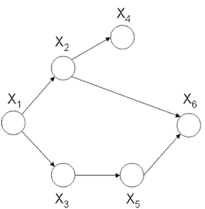
If we use Theorem 1 it can be seen that the joint probability density function for Figure 7 can be written as follows:
Once again, we can apply the Chain Rule and then the Markov Property and arrive at the same result.
Independence
Marginal independence
We can say that [math]\displaystyle{ X_A }[/math] is marginally independent of [math]\displaystyle{ X_B }[/math] if:
Conditional independence
We can say that [math]\displaystyle{ X_A }[/math] is conditionally independent of [math]\displaystyle{ X_B }[/math] given [math]\displaystyle{ X_C }[/math] if:
Note: Both equations are equivalent. Aside: Before we move on further, we first define the following terms:
- I is defined as an ordering for the nodes in graph C.
- For each [math]\displaystyle{ i \in V }[/math], [math]\displaystyle{ V_i }[/math] is defined as a set of all nodes that appear earlier than i excluding its parents [math]\displaystyle{ \pi_i }[/math].
Let us consider the example of the six node figure given above (Figure 7). We can define [math]\displaystyle{ I }[/math] as follows:
We can then easily compute [math]\displaystyle{ V_i }[/math] for say [math]\displaystyle{ i=3,6 }[/math].
while [math]\displaystyle{ \pi_i }[/math] for [math]\displaystyle{ i=3,6 }[/math] will be.
We would be interested in finding the conditional independence between random variables in this graph. We know [math]\displaystyle{ X_i \perp X_{v_i} | X_{\pi_i} }[/math] for each [math]\displaystyle{ i }[/math]. In other words, given its parents the node is independent of all earlier nodes. So:
[math]\displaystyle{ X_1 \perp \phi | \phi }[/math],
[math]\displaystyle{ X_2 \perp \phi | X_1 }[/math],
[math]\displaystyle{ X_3 \perp X_2 | X_1 }[/math],
[math]\displaystyle{ X_4 \perp \{X_1,X_3\} | X_2 }[/math],
[math]\displaystyle{ X_5 \perp \{X_1,X_2,X_4\} | X_3 }[/math],
[math]\displaystyle{ X_6 \perp \{X_1,X_3,X_4\} | \{X_2,X_5\} }[/math]
To illustrate why this is true we can take a simple example. Show that:
Proof: first, we know [math]\displaystyle{ P(X_1,X_2,X_3,X_4,X_5,X_6) = P(X_1)P(X_2|X_1)P(X_3|X_1)P(X_4|X_2)P(X_5|X_3)P(X_6|X_5,X_2)\,\! }[/math]
then
The other conditional independences can be proven through a similar process.
Sampling
Even if using graphical models helps a lot facilitate obtaining the joint probability, exact inference is not always feasible. Exact inference is feasible in small to medium-sized networks only. Exact inference consumes such a long time in large networks. Therefore, we resort to approximate inference techniques which are much faster and usually give pretty good results.
In sampling, random samples are generated and values of interest are computed from samples, not original work.
As an input you have a Bayesian network with set of nodes [math]\displaystyle{ X\,\! }[/math]. The sample taken may include all variables (except evidence E) or a subset. Sample schemas dictate how to generate samples (tuples). Ideally samples are distributed according to [math]\displaystyle{ P(X|E)\,\! }[/math]
Some sampling algorithms:
- Forward Sampling
- Likelihood weighting
- Gibbs Sampling (MCMC)
- Blocking
- Rao-Blackwellised
- Importance Sampling
Bayes Ball
The Bayes Ball algorithm can be used to determine if two random variables represented in a graph are independent. The algorithm can show that either two nodes in a graph are independent OR that they are not necessarily independent. The Bayes Ball algorithm can not show that two nodes are dependent. In other word it provides some rules which enables us to do this task using the graph without the need to use the probability distributions. The algorithm will be discussed further in later parts of this section.
Canonical Graphs
In order to understand the Bayes Ball algorithm we need to first introduce 3 canonical graphs. Since our graphs are acyclic, we can represent them using these 3 canonical graphs.
Markov Chain (also called serial connection)
In the following graph (Figure 8 X is independent of Z given Y.
We say that: [math]\displaystyle{ X }[/math] [math]\displaystyle{ \perp }[/math] [math]\displaystyle{ Z }[/math] [math]\displaystyle{ | }[/math] [math]\displaystyle{ Y }[/math]

We can prove this independence:
Where
Markov chains are an important class of distributions with applications in communications, information theory and image processing. They are suitable to model memory in phenomenon. For example suppose we want to study the frequency of appearance of English letters in a text. Most likely when "q" appears, the next letter will be "u", this shows dependency between these letters. Markov chains are suitable model this kind of relations.

Markov chains play a significant role in biological applications. It is widely used in the study of carcinogenesis (initiation of cancer formation). A gene has to undergo several mutations before it becomes cancerous, which can be addressed through Markov chains. An example is given in Figure 8a which shows only two gene mutations.
Hidden Cause (diverging connection)
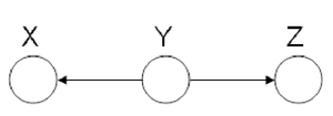
In the Hidden Cause case we can say that X is independent of Z given Y. In this case Y is the hidden cause and if it is known then Z and X are considered independent.
We say that: [math]\displaystyle{ X }[/math] [math]\displaystyle{ \perp }[/math] [math]\displaystyle{ Z }[/math] [math]\displaystyle{ | }[/math] [math]\displaystyle{ Y }[/math]
The proof of the independence:
The Hidden Cause case is best illustrated with an example:
In Figure 10 it can be seen that both "Shoe Size" and "Grey Hair" are dependant on the age of a person. The variables of "Shoe size" and "Grey hair" are dependent in some sense, if there is no "Age" in the picture. Without the age information we must conclude that those with a large shoe size also have a greater chance of having gray hair. However, when "Age" is observed, there is no dependence between "Shoe size" and "Grey hair" because we can deduce both based only on the "Age" variable.
Explaining-Away (converging connection)
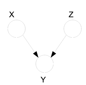
Finally, we look at the third type of canonical graph: Explaining-Away Graphs. This type of graph arises when a phenomena has multiple explanations. Here, the conditional independence statement is actually a statement of marginal independence: [math]\displaystyle{ X \perp Z }[/math]. This type of graphs is also called "V-structure" or "V-shape" because of its illustration (Fig. 11).
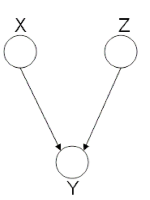
In these types of scenarios, variables X and Z are independent. However, once the third variable Y is observed, X and Z become dependent (Fig. 11).
To clarify these concepts, suppose Bob and Mary are supposed to meet for a noontime lunch. Consider the following events:
If Mary is late, then she could have been kidnapped by aliens. Alternatively, Bob may have forgotten to adjust his watch for daylight savings time, making him early. Clearly, both of these events are independent. Now, consider the following probabilities:
We expect [math]\displaystyle{ P( late = 1 ) \lt P( aliens = 1 ~|~ late = 1 ) }[/math] since [math]\displaystyle{ P( aliens = 1 ~|~ late = 1 ) }[/math] does not provide any information regarding Bob's watch. Similarly, we expect [math]\displaystyle{ P( aliens = 1 ~|~ late = 1 ) \lt P( aliens = 1 ~|~ late = 1, watch = 0 ) }[/math]. Since [math]\displaystyle{ P( aliens = 1 ~|~ late = 1 ) \neq P( aliens = 1 ~|~ late = 1, watch = 0 ) }[/math], aliens and watch are not independent given late. To summarize,
- If we do not observe late, then aliens [math]\displaystyle{ ~\perp~ watch }[/math] ([math]\displaystyle{ X~\perp~ Z }[/math])
- If we do observe late, then aliens [math]\displaystyle{ ~\cancel{\perp}~ watch ~|~ late }[/math] ([math]\displaystyle{ X ~\cancel{\perp}~ Z ~|~ Y }[/math])
Bayes Ball Algorithm
Goal: We wish to determine whether a given conditional statement such as [math]\displaystyle{ X_{A} ~\perp~ X_{B} ~|~ X_{C} }[/math] is true given a directed graph.
The algorithm is as follows:
- Shade nodes, [math]\displaystyle{ ~X_{C}~ }[/math], that are conditioned on, i.e. they have been observed.
- Assuming that the initial position of the ball is [math]\displaystyle{ ~X_{A}~ }[/math]:
- If the ball cannot reach [math]\displaystyle{ ~X_{B}~ }[/math], then the nodes [math]\displaystyle{ ~X_{A}~ }[/math] and [math]\displaystyle{ ~X_{B}~ }[/math] must be conditionally independent.
- If the ball can reach [math]\displaystyle{ ~X_{B}~ }[/math], then the nodes [math]\displaystyle{ ~X_{A}~ }[/math] and [math]\displaystyle{ ~X_{B}~ }[/math] are not necessarily independent.
The biggest challenge in the Bayes Ball Algorithm is to determine what happens to a ball going from node X to node Z as it passes through node Y. The ball could continue its route to Z or it could be blocked. It is important to note that the balls are allowed to travel in any direction, independent of the direction of the edges in the graph.
We use the canonical graphs previously studied to determine the route of a ball traveling through a graph. Using these three graphs, we establish the Bayes ball rules which can be extended for more graphical models.
Markov Chain (serial connection)
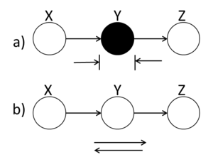
A ball traveling from X to Z or from Z to X will be blocked at node Y if this node is shaded. Alternatively, if Y is unshaded, the ball will pass through.
In (Fig. 12(a)), X and Z are conditionally independent ( [math]\displaystyle{ X ~\perp~ Z ~|~ Y }[/math] ) while in (Fig.12(b)) X and Z are not necessarily independent.
Hidden Cause (diverging connection)
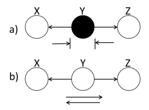
A ball traveling through Y will be blocked at Y if it is shaded. If Y is unshaded, then the ball passes through.
(Fig. 13(a)) demonstrates that X and Z are conditionally independent when Y is shaded.
Explaining-Away (converging connection)
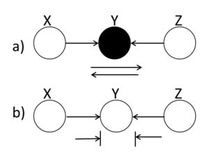
Unlike the last two cases in which the Bayes ball rule was intuitively understandable, in this case a ball traveling through Y is blocked when Y is UNSHADED!. If Y is shaded, then the ball passes through. Hence, X and Z are conditionally independent when Y is unshaded.
Bayes Ball Examples
Example 1
In this first example, we wish to identify the behavior of leaves in the graphical models using two-nodes graphs. Let a ball be going from X to Y in two-node graphs. To employ the Bayes ball method mentioned above, we have to implicitly add one extra node to the two-node structure since we introduced the Bayes rules for three nodes configuration. We add the third node exactly symmetric to node X with respect to node Y. For example in (Fig. 15) (a) we can think of a hidden node in the right hand side of node Y with a hidden arrow from the hidden node to Y. Then, we are able to utilize the Bayes ball method considering the fact that a ball thrown from X cannot reach Y, and thus it will be blocked. On the contrary, following the same rule in (Fig. 15) (b) turns out that if there was a hidden node in right hand side of Y, a ball could pass from X to that hidden node according to explaining-away structure. Of course, there is no real node and in this case we conventionally say that the ball will be bounced back to node X.
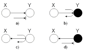
Finally, for the last two graphs, we used the rules of the Hidden Cause Canonical Graph (Fig. 13). In (c), the ball passes through Y while in (d), the ball is blocked at Y.
Example 2
Suppose your home is equipped with an alarm system. There are two possible causes for the alarm to ring:
- Your house is being burglarized
- There is an earthquake
Hence, we define the following events:
The burglary and earthquake events are independent
if the alarm does not ring. However, if the alarm does ring, then
the burglary and the earthquake events are not
necessarily independent. Also, if the alarm rings then it is
more possible that a police report will be issued.
We can use the Bayes Ball Algorithm to deduce conditional independence properties from the graph. Firstly, consider figure (16(a)) and assume we are trying to determine whether there is conditional independence between the burglary and earthquake events. In figure (\ref{fig:AlarmExample1}(a)), a ball starting at the burglary event is blocked at the alarm node.
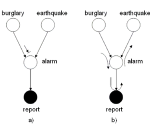
Nonetheless, this does not prove that the burglary and earthquake events are independent. Indeed, (Fig. 16(b)) disproves this as we have found an alternate path from burglary to earthquake passing through report. It follows that [math]\displaystyle{ burglary ~\cancel{\amalg}~ earthquake ~|~ report }[/math]
Example 3
Referring to figure (Fig. 17), we wish to determine whether the following conditional probabilities are true:

To determine if the conditional probability Eq.\ref{eq:c1} is true, we shade node [math]\displaystyle{ X_{2} }[/math]. This blocks balls traveling from [math]\displaystyle{ X_{1} }[/math] to [math]\displaystyle{ X_{3} }[/math] and proves that Eq.\ref{eq:c1} is valid.
After shading nodes [math]\displaystyle{ X_{3} }[/math] and [math]\displaystyle{ X_{4} }[/math] and applying the Bayes Balls Algorithm}, we find that the ball travelling from [math]\displaystyle{ X_{1} }[/math] to [math]\displaystyle{ X_{5} }[/math] is blocked at [math]\displaystyle{ X_{3} }[/math]. Similarly, a ball going from [math]\displaystyle{ X_{5} }[/math] to [math]\displaystyle{ X_{1} }[/math] is blocked at [math]\displaystyle{ X_{4} }[/math]. This proves that Eq.\ref{eq:c2 also holds.
Example 4

Consider figure (Fig. 18). Using the Bayes Ball Algorithm we wish to determine if each of the following statements are valid:
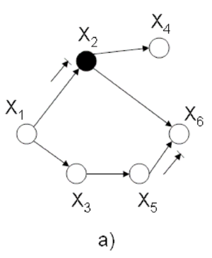
To disprove Eq.\ref{eq:c3}, we must find a path from [math]\displaystyle{ X_{4} }[/math] to [math]\displaystyle{ X_{1} }[/math] and [math]\displaystyle{ X_{3} }[/math] when [math]\displaystyle{ X_{2} }[/math] is shaded (Refer to Fig. 19(a)). Since there is no route from [math]\displaystyle{ X_{4} }[/math] to [math]\displaystyle{ X_{1} }[/math] and [math]\displaystyle{ X_{3} }[/math] we conclude that Eq.\ref{eq:c3} is true.
Similarly, we can show that there does not exist a path between [math]\displaystyle{ X_{1} }[/math] and [math]\displaystyle{ X_{6} }[/math] when [math]\displaystyle{ X_{2} }[/math] and [math]\displaystyle{ X_{3} }[/math] are shaded (Refer to Fig.19(b)). Hence, Eq.\ref{eq:c4} is true.
Finally, (Fig. 19(c)) shows that there is a route from [math]\displaystyle{ X_{2} }[/math] to [math]\displaystyle{ X_{3} }[/math] when [math]\displaystyle{ X_{1} }[/math] and [math]\displaystyle{ X_{6} }[/math] are shaded. This proves that the statement \ref{eq:c4} is false.
Theorem 2.
Define [math]\displaystyle{ p(x_{v}) = \prod_{i=1}^{n}{p(x_{i} ~|~ x_{\pi_{i}})} }[/math] to be the factorization as a multiplication of some local probability of a directed graph.
Let [math]\displaystyle{ D_{1} = \{ p(x_{v}) = \prod_{i=1}^{n}{p(x_{i} ~|~ x_{\pi_{i}})}\} }[/math]
Let [math]\displaystyle{ D_{2} = \{ p(x_{v}): }[/math]satisfy all conditional independence statements associated with a graph [math]\displaystyle{ \} }[/math].
Then [math]\displaystyle{ D_{1} = D_{2} }[/math].
Example 5
Given the following Bayesian network (Fig.19 ): Determine whether the following statements are true or false?
a.) [math]\displaystyle{ x4\perp \{x1,x3\} }[/math]
Ans. True
b.) [math]\displaystyle{ x1\perp x6\{x2,x3\} }[/math]
Ans. True
c.) [math]\displaystyle{ x2\perp x3 \{x1,x6\} }[/math]
Ans. False
Undirected Graphical Model
Generally, the graphical model is divided into two major classes, directed graphs and undirected graphs. Directed graphs and its characteristics was described previously. In this section we discuss undirected graphical model which is also known as Markov random fields. In some applications there are relations between variables but these relation are bilateral and we don't encounter causality. For example consider a natural image. In natural images the value of a pixel has correlations with neighboring pixel values but this is bilateral and not a causality relations. Markov random fields are suitable to model such processes and have found applications in fields such as vision and image processing.We can define an undirected graphical model with a graph [math]\displaystyle{ G = (V, E) }[/math] where [math]\displaystyle{ V }[/math] is a set of vertices corresponding to a set of random variables and [math]\displaystyle{ E }[/math] is a set of undirected edges as shown in (Fig.20)
Conditional independence
For directed graphs Bayes ball method was defined to determine the conditional independence properties of a given graph. We can also employ the Bayes ball algorithm to examine the conditional independency of undirected graphs. Here the Bayes ball rule is simpler and more intuitive. Considering (Fig.21) , a ball can be thrown either from x to z or from z to x if y is not observed. In other words, if y is not observed a ball thrown from x can reach z and vice versa. On the contrary, given a shaded y, the node can block the ball and make x and z conditionally independent. With this definition one can declare that in an undirected graph, a node is conditionally independent of non-neighbors given neighbors. Technically speaking, [math]\displaystyle{ X_A }[/math] is independent of [math]\displaystyle{ X_C }[/math] given [math]\displaystyle{ X_B }[/math] if the set of nodes [math]\displaystyle{ X_B }[/math] separates the nodes [math]\displaystyle{ X_A }[/math] from the nodes [math]\displaystyle{ X_C }[/math]. Hence, if every path from a node in [math]\displaystyle{ X_A }[/math] to a node in [math]\displaystyle{ X_C }[/math] includes at least one node in [math]\displaystyle{ X_B }[/math], then we claim that [math]\displaystyle{ X_A \perp X_c | X_B }[/math].
Question
Is it possible to convert undirected models to directed models or vice versa?
In order to answer this question, consider (Fig.22 ) which illustrates an undirected graph with four nodes - [math]\displaystyle{ X }[/math], [math]\displaystyle{ Y }[/math],[math]\displaystyle{ Z }[/math] and [math]\displaystyle{ W }[/math]. We can define two facts using Bayes ball method:
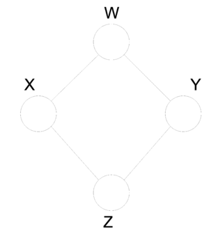
It is simple to see there is no directed graph satisfying both conditional independence properties. Recalling that directed graphs are acyclic, converting undirected graphs to directed graphs result in at least one node in which the arrows are inward-pointing(a v structure). Without loss of generality we can assume that node [math]\displaystyle{ Z }[/math] has two inward-pointing arrows. By conditional independence semantics of directed graphs, we have [math]\displaystyle{ X \perp Y|W }[/math], yet the [math]\displaystyle{ X \perp Y|\{W,Z\} }[/math] property does not hold. On the other hand, (Fig.23 ) depicts a directed graph which is characterized by the singleton independence statement [math]\displaystyle{ X \perp Y }[/math]. There is no undirected graph on three nodes which can be characterized by this singleton statement. Basically, if we consider the set of all distribution over [math]\displaystyle{ n }[/math] random variables, a subset of which can be represented by directed graphical models while there is another subset which undirected graphs are able to model that. There is a narrow intersection region between these two subsets in which probabilistic graphical models may be represented by either directed or undirected graphs.
Parameterization
Having undirected graphical models, we would like to obtain "local" parameterization like what we did in the case of directed graphical models. For directed graphical models, "local" had the interpretation of a set of node and its parents, [math]\displaystyle{ \{i, \pi_i\} }[/math]. The joint probability and the marginals are defined as a product of such local probabilities which was inspired from the chain rule in the probability theory. In undirected GMs "local" functions cannot be represented using conditional probabilities, and we must abandon conditional probabilities altogether. Therefore, the factors do not have probabilistic interpretation any more, but we can choose the "local" functions arbitrarily. However, any "local" function for undirected graphical models should satisfy the following condition: - Consider [math]\displaystyle{ X_i }[/math] and [math]\displaystyle{ X_j }[/math] that are not linked, they are conditionally independent given all other nodes. As a result, the "local" function should be able to do the factorization on the joint probability such that [math]\displaystyle{ X_i }[/math] and [math]\displaystyle{ X_j }[/math] are placed in different factors.
It can be shown that definition of local functions based only a node and its corresponding edges (similar to directed graphical models) is not tractable and we need to follow a different approach. Before defining the "local" functions, we have to introduce a new terminology in graph theory called clique. Clique is a subset of fully connected nodes in a graph G. Every node in the clique C is directly connected to every other node in C. In addition, maximal clique is a clique where if any other node from the graph G is added to it then the new set is no longer a clique. Consider the undirected graph shown in (Fig. 24), we can list all the cliques as follow:
- [math]\displaystyle{ \{X_1, X_3\} }[/math] - [math]\displaystyle{ \{X_1, X_2\} }[/math] - [math]\displaystyle{ \{X_3, X_5\} }[/math] - [math]\displaystyle{ \{X_2, X_4\} }[/math] - [math]\displaystyle{ \{X_5, X_6\} }[/math] - [math]\displaystyle{ \{X_2, X_5\} }[/math] - [math]\displaystyle{ \{X_2, X_5, X_6\} }[/math]
According to the definition, [math]\displaystyle{ \{X_2,X_5\} }[/math] is not a maximal clique since we can add one more node, [math]\displaystyle{ X_6 }[/math] and still have a clique. Let C be set of all maximal cliques in [math]\displaystyle{ G(V, E) }[/math]:
where in aforementioned example [math]\displaystyle{ c_1 }[/math] would be [math]\displaystyle{ \{X_1, X_3\} }[/math], and so on. We define the joint probability over all nodes as:
where [math]\displaystyle{ \psi_{c_i} (x_{c_i}) }[/math] is an arbitrarily function with some restrictions. This function is not necessarily probability and is defined over each clique. There are only two restrictions for this function, non-negative and real-valued. Usually [math]\displaystyle{ \psi_{c_i} (x_{c_i}) }[/math] is called potential function. The [math]\displaystyle{ Z }[/math] is normalization factor and determined by:
As a matter of fact, normalization factor, [math]\displaystyle{ Z }[/math], is not very important since in most of the time is canceled out during computation. For instance, to calculate conditional probability [math]\displaystyle{ P(X_A | X_B) }[/math], [math]\displaystyle{ Z }[/math] is crossed out between the nominator [math]\displaystyle{ P(X_A, X_B) }[/math] and the denominator [math]\displaystyle{ P(X_B) }[/math].
As was mentioned above, sum-product of the potential functions determines the joint probability over all nodes. Because of the fact that potential functions are arbitrarily defined, assuming exponential functions for [math]\displaystyle{ \psi_{c_i} (x_{c_i}) }[/math] simplifies and reduces the computations. Let potential function be:
the joint probability is given by:
-
There is a lot of information contained in the joint probability distribution [math]\displaystyle{ P(x_{V}) }[/math]. We define 6 tasks listed bellow that we would like to accomplish with various algorithms for a given distribution [math]\displaystyle{ P(x_{V}) }[/math].
Tasks:
- Marginalization
Given [math]\displaystyle{ P(x_{V}) }[/math] find [math]\displaystyle{ P(x_{A}) }[/math]
\underline{ex.} Given [math]\displaystyle{ P(x_1, x_2, ... , x_6) }[/math] find [math]\displaystyle{ P(x_2, x_6) }[/math]
- Conditioning
Given [math]\displaystyle{ P(x_V) }[/math] find [math]\displaystyle{ P(x_A|x_B) = \frac{P(x_A, x_B)}{P(x_B)} }[/math] .
- Evaluation
Evaluate the probability for a certain configuration.
- Completion
Compute the most probable configuration. In other words, which of the [math]\displaystyle{ P(x_A|x_B) }[/math] is the largest for a specific combinations of [math]\displaystyle{ A }[/math] and [math]\displaystyle{ B }[/math].
- Simulation
Generate a random configuration for [math]\displaystyle{ P(x_V) }[/math] .
- Learning
We would like to find parameters for [math]\displaystyle{ P(x_V) }[/math] .
Exact Algorithms:
We will be looking at three exact algorithms. An exact algorithm is an algorithm that will find the exact answer to one of the above tasks. The main disadvantage to the exact algorithms approach is that for large graphs which have a large number of nodes these algorithms take a long time to produce a result. When this occurs we can use inexact algorithms to more efficiently find a useful estimate.
- Elimination
- Sum-Product
- Max-Product
- Junction Tree
{{
Template:namespace detect
| type = style | image = | imageright = | style = | textstyle = | text = This article may require cleanup to meet Wikicoursenote's quality standards. The specific problem is: I think a large graph or a large number of the nodes is not the main case that these algorithms doesn't work. These algorithm will lead to expensive computation when the graph is not sparse, i.e., the graph posses a lot of edges. In such cases we need to somehow simply and use approximate methods.. Please improve this article if you can. (October 2011) | small = | smallimage = | smallimageright = | smalltext = }}
Elimination Algorithm
In this section we will see how we could overcome the problem of probabilistic inference on graphical models. In other words, we discuss the problem of computing conditional and marginal probabilities in graphical models.
Elimination Algorithm on Directed Graphs
First we assume that E and F are disjoint subsets of the node indices of a graphical model, i.e. [math]\displaystyle{ X_E }[/math] and [math]\displaystyle{ X_F }[/math] are disjoint subsets of the random variables. Given a graph G =(V,E), we aim to calculate [math]\displaystyle{ p(x_F | x_E) }[/math] where [math]\displaystyle{ X_E }[/math] and [math]\displaystyle{ X_F }[/math] represents evidence and query nodes, respectively. Here and in this section [math]\displaystyle{ X_F }[/math] should be only one node; however, later on a more powerful inference method will be introduced which is able to make inference on multi-variables. In order to compute [math]\displaystyle{ p(x_F | x_E) }[/math] we have to first marginalize the joint probability on nodes which are neither [math]\displaystyle{ X_F }[/math] nor [math]\displaystyle{ X_E }[/math] denoted by [math]\displaystyle{ R = V - ( E U F) }[/math].
which can be further marginalized to yield [math]\displaystyle{ p(E) }[/math]:
and then the desired conditional probability is given by:
Example
Let assume that we are interested in [math]\displaystyle{ p(x_1 | \bar{x_6)} }[/math] in (Fig. 21) where [math]\displaystyle{ x_6 }[/math] is an observation of [math]\displaystyle{ X_6 }[/math] , and thus we may assume that it is a constant. According to the rule mentioned above we have to marginalized the joint probability over non-evidence and non-query nodes:
where to simplify the notations we define [math]\displaystyle{ m_5(x_2, x_3) }[/math] which is the result of the last summation. The last summation is over [math]\displaystyle{ x_5 }[/math] , and thus the result is only depend on [math]\displaystyle{ x_2 }[/math] and [math]\displaystyle{ x_3 }[/math]. In particular, let [math]\displaystyle{ m_i(x_{s_i}) }[/math] denote the expression that arises from performing the [math]\displaystyle{ \sum_{x_i} }[/math], where [math]\displaystyle{ x_{S_i} }[/math] are the variables, other than [math]\displaystyle{ x_i }[/math], that appear in the summand. Continuing the derivations we have:
Therefore, the conditional probability is given by:
At the beginning of our computation we had the assumption which says [math]\displaystyle{ X_6 }[/math] is observed, and thus the notation [math]\displaystyle{ \bar{x_6} }[/math] was used to express this fact. Let [math]\displaystyle{ X_i }[/math] be an evidence node whose observed value is [math]\displaystyle{ \bar{x_i} }[/math], we define an evidence potential function, [math]\displaystyle{ \delta(x_i, \bar{x_i}) }[/math], which its value is one if [math]\displaystyle{ x_i = \bar{x_i} }[/math] and zero elsewhere. This function allows us to use summation over [math]\displaystyle{ x_6 }[/math] yielding:
We can define an algorithm to make inference on directed graphs using elimination techniques. Let E and F be an evidence set and a query node, respectively. We first choose an elimination ordering I such that F appears last in this ordering. The following figure shows the steps required to perform the elimination algorithm for probabilistic inference on directed graphs:
ELIMINATE (G,E,F)

INITIALIZE (G,F)

EVIDENCE(E)

UPDATE(G)
NORMALIZE(F)
INITIALIZE(G,F)

Choose an ordering [math]\displaystyle{ I }[/math] such that [math]\displaystyle{ F }[/math] appear last
- For each node [math]\displaystyle{ X_i }[/math] in [math]\displaystyle{ V }[/math]
- Place [math]\displaystyle{ p(x_i|x_{\pi_i}) }[/math] on the active list
- End
EVIDENCE(E)
- For each [math]\displaystyle{ i }[/math] in [math]\displaystyle{ E }[/math]
- Place [math]\displaystyle{ \delta(x_i|\overline{x_i}) }[/math] on the active list
- End
Update(G)
- For each [math]\displaystyle{ i }[/math] in [math]\displaystyle{ I }[/math]
- Find all potentials from the active list that reference [math]\displaystyle{ x_i }[/math] and remove them from the active list
- Let [math]\displaystyle{ \phi_i(x_Ti) }[/math] denote the product of these potentials
- Let [math]\displaystyle{ m_i(x_Si)=\sum_{x_i}\phi_i(x_Ti) }[/math]
- Place [math]\displaystyle{ m_i(x_Si) }[/math] on the active list
- End
Normalize(F)
- [math]\displaystyle{ p(x_F|\overline{x_E}) }[/math] ← [math]\displaystyle{ \phi_F(x_F)/\sum_{x_F}\phi_F(x_F) }[/math]
Example:
For the graph in figure 21 [math]\displaystyle{ G =(V,''E'') }[/math]. Consider once again that node [math]\displaystyle{ x_1 }[/math] is the query node and [math]\displaystyle{ x_6 }[/math] is the evidence node.
[math]\displaystyle{ I = \left\{6,5,4,3,2,1\right\} }[/math] (1 should be the last node, ordering is crucial)

We must now create an active list. There are two rules that must be followed in order to create this list.
- For i[math]\displaystyle{ \in{V} }[/math] place [math]\displaystyle{ p(x_i|x_{\pi_i}) }[/math] in active list.
- For i[math]\displaystyle{ \in }[/math]{E} place [math]\displaystyle{ \delta(x_i|\overline{x_i}) }[/math] in active list.
Here, our active list is: [math]\displaystyle{ p(x_1), p(x_2|x_1), p(x_3|x_1), p(x_4|x_2), p(x_5|x_3),\underbrace{p(x_6|x_2, x_5)\delta{(\overline{x_6},x_6)}}_{\phi_6(x_2,x_5, x_6), \sum_{x6}{\phi_6}=m_{6}(x2,x5) } }[/math]
We first eliminate node [math]\displaystyle{ X_6 }[/math]. We place [math]\displaystyle{ m_{6}(x_2,x_5) }[/math] on the active list, having removed [math]\displaystyle{ X_6 }[/math]. We now eliminate [math]\displaystyle{ X_5 }[/math].
Likewise, we can also eliminate [math]\displaystyle{ X_4, X_3, X_2 }[/math](which yields the unnormalized conditional probability [math]\displaystyle{ p(x_1|\overline{x_6}) }[/math] and [math]\displaystyle{ X_1 }[/math]. Then it yields [math]\displaystyle{ m_1 = \sum_{x_1}{\phi_1(x_1)} }[/math] which is the normalization factor, [math]\displaystyle{ p(\overline{x_6}) }[/math].
Elimination Algorithm on Undirected Graphs
The first task is to find the maximal cliques and their associated potential functions.
maximal clique: [math]\displaystyle{ \left\{x_1, x_2\right\} }[/math], [math]\displaystyle{ \left\{x_1, x_3\right\} }[/math], [math]\displaystyle{ \left\{x_2, x_4\right\} }[/math], [math]\displaystyle{ \left\{x_3, x_5\right\} }[/math], [math]\displaystyle{ \left\{x_2,x_5,x_6\right\} }[/math]
potential functions: [math]\displaystyle{ \varphi{(x_1,x_2)},\varphi{(x_1,x_3)},\varphi{(x_2,x_4)}, \varphi{(x_3,x_5)} }[/math] and [math]\displaystyle{ \varphi{(x_2,x_3,x_6)} }[/math]
[math]\displaystyle{ p(x_1|\overline{x_6})=p(x_1,\overline{x_6})/p(\overline{x_6})\cdots\cdots\cdots\cdots\cdots(*) }[/math]
[math]\displaystyle{ p(x_1,x_6)=\frac{1}{Z}\sum_{x_2,x_3,x_4,x_5,x_6}\varphi{(x_1,x_2)}\varphi{(x_1,x_3)}\varphi{(x_2,x_4)}\varphi{(x_3,x_5)}\varphi{(x_2,x_3,x_6)}\delta{(x_6,\overline{x_6})} }[/math]
The [math]\displaystyle{ \frac{1}{Z} }[/math] looks crucial, but in fact it has no effect because for (*) both the numerator and the denominator have the [math]\displaystyle{ \frac{1}{Z} }[/math] term. So in this case we can just cancel it.
The general rule for elimination in an undirected graph is that we can remove a node as long as we connect all of the parents of that node together. Effectively, we form a clique out of the parents of that node.
The algorithm used to eliminate nodes in an undirected graph is:
UndirectedGraphElimination(G,l)
- For each node [math]\displaystyle{ X_i }[/math] in [math]\displaystyle{ I }[/math]
- Connect all of the remaining neighbours of [math]\displaystyle{ X_i }[/math]
- Remove [math]\displaystyle{ X_i }[/math] from the graph
- End
Example:
For the graph G in figure 24
when we remove x1, G becomes as in figure 25
while if we remove x2, G becomes as in figure 26
An interesting thing to point out is that the order of the elimination matters a great deal. Consider the two results. If we remove one node the graph complexity is slightly reduced. But if we try to remove another node the complexity is significantly increased. The reason why we even care about the complexity of the graph is because the complexity of a graph denotes the number of calculations that are required to answer questions about that graph. If we had a huge graph with thousands of nodes the order of the node removal would be key in the complexity of the algorithm. Unfortunately, there is no efficient algorithm that can produce the optimal node removal order such that the elimination algorithm would run quickly. If we remove one of the leaf first, then the largest clique is two and computational complexity is of order [math]\displaystyle{ N^2 }[/math]. And removing the center node gives the largest clique size to be five and complexity is of order [math]\displaystyle{ N^5 }[/math]. Hence, it is very hard to find an optimal ordering, due to which this is an NP problem.
Moralization
So far we have shown how to use elimination to successively remove nodes from an undirected graph. We know that this is useful in the process of marginalization. We can now turn to the question of what will happen when we have a directed graph. It would be nice if we could somehow reduce the directed graph to an undirected form and then apply the previous elimination algorithm. This reduction is called moralization and the graph that is produced is called a moral graph.
To moralize a graph we first need to connect the parents of each node together. This makes sense intuitively because the parents of a node need to be considered together in the undirected graph and this is only done if they form a type of clique. By connecting them together we create this clique.
After the parents are connected together we can just drop the orientation on the edges in the directed graph. By removing the directions we force the graph to become undirected.
The previous elimination algorithm can now be applied to the new moral graph. We can do this by assuming that the probability functions in directed graph [math]\displaystyle{ P(x_i|\pi_{x_i}) }[/math] are the same as the mass functions from the undirected graph. [math]\displaystyle{ \psi_{c_i}(c_{x_i}) }[/math]
Example:
I = [math]\displaystyle{ \left\{x_6,x_5,x_4,x_3,x_2,x_1\right\} }[/math]
When we moralize the directed graph in figure 27, we obtain the
undirected graph in figure 28.
Elimination Algorithm on Trees
Definition of a tree:
A tree is an undirected graph in which any two vertices are connected by exactly one simple path. In other words, any connected graph without cycles is a tree.
If we have a directed graph then we must moralize it first. If the moral graph is a tree then the directed graph is also considered a tree.
Belief Propagation Algorithm (Sum Product Algorithm)
One of the main disadvantages to the elimination algorithm is that the ordering of the nodes defines the number of calculations that are required to produce a result. The optimal ordering is difficult to calculate and without a decent ordering the algorithm may become very slow. In response to this we can introduce the sum product algorithm. It has one major advantage over the elimination algorithm: it is faster. The sum product algorithm has the same complexity when it has to compute the probability of one node as it does to compute the probability of all the nodes in the graph. Unfortunately, the sum product algorithm also has one disadvantage. Unlike the elimination algorithm it can not be used on any graph. The sum product algorithm works only on trees.
For undirected graphs if there is only one path between any two pair of nodes then that graph is a tree (Fig.29). If we have a directed graph then we must moralize it first. If the moral graph is a tree then the directed graph is also considered a tree (Fig.30).
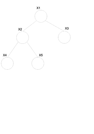
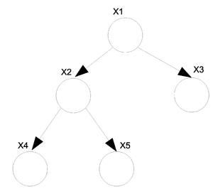
For the undirected graph [math]\displaystyle{ G(v, \varepsilon) }[/math] (Fig.30) we can write the joint probability distribution function in the following way.
We know that in general we can not convert a directed graph into an undirected graph. There is however an exception to this rule when it comes to trees. In the case of a directed tree there is an algorithm that allows us to convert it to an undirected tree with the same properties.
Take the above example (Fig.30) of a directed tree. We can write the joint probability distribution function as:
If we want to convert this graph to the undirected form shown in (Fig. \ref{fig:UnDirTree}) then we can use the following set of rules. \begin{thinlist}
- If [math]\displaystyle{ \gamma }[/math] is the root then: [math]\displaystyle{ \psi(x_\gamma) = P(x_\gamma) }[/math].
- If [math]\displaystyle{ \gamma }[/math] is NOT the root then: [math]\displaystyle{ \psi(x_\gamma) = 1 }[/math].
- If [math]\displaystyle{ \left\lbrace i \right\rbrace }[/math] = [math]\displaystyle{ \pi_j }[/math] then: [math]\displaystyle{ \psi(x_i, x_j) = P(x_j | x_i) }[/math].
\end{thinlist} So now we can rewrite the above equation for (Fig.30) as:
Elimination Algorithm on a Tree
We will derive the Sum-Product algorithm from the point of view of the Eliminate algorithm. To marginalize [math]\displaystyle{ x_1 }[/math] in Fig.31,
where,
which is essentially (potential of the node)[math]\displaystyle{ \times }[/math](potential of the edge)[math]\displaystyle{ \times }[/math](message from the child).
The term "[math]\displaystyle{ m_{ji}(x_i) }[/math]" represents the intermediate factor between the eliminated variable, j, and the remaining neighbor of the variable, i. Thus, in the above case, we will use [math]\displaystyle{ m_{53}(x_3) }[/math] to denote [math]\displaystyle{ m_5(x_3) }[/math], [math]\displaystyle{ m_{42}(x_2) }[/math] to denote [math]\displaystyle{ m_4(x_2) }[/math], and [math]\displaystyle{ m_{32}(x_2) }[/math] to denote [math]\displaystyle{ m_3(x_2) }[/math]. We refer to the intermediate factor [math]\displaystyle{ m_{ji}(x_i) }[/math] as a "message" that j sends to i. (Fig. \ref{fig:TreeStdEx})
In general,
Note: It is important to know that BP algorithm gives us the exact solution only if the graph is a tree, however experiments have shown that BP leads to acceptable approximate answer even when the graphs has some loops.
Elimination To Sum Product Algorithm
The Sum-Product algorithm allows us to compute all marginals in the tree by passing messages inward from the leaves of the tree to an (arbitrary) root, and then passing it outward from the root to the leaves, again using the above equation at each step. The net effect is that a single message will flow in both directions along each edge. (See Fig.32) Once all such messages have been computed using the above equation, we can compute desired marginals. One of the major advantages of this algorithm is that messages can be reused which reduces the computational cost heavily.
As shown in Fig.32, to compute the marginal of [math]\displaystyle{ X_1 }[/math] using elimination, we eliminate [math]\displaystyle{ X_5 }[/math], which involves computing a message [math]\displaystyle{ m_{53}(x_3) }[/math], then eliminate [math]\displaystyle{ X_4 }[/math] and [math]\displaystyle{ X_3 }[/math] which involves messages [math]\displaystyle{ m_{32}(x_2) }[/math] and [math]\displaystyle{ m_{42}(x_2) }[/math]. We subsequently eliminate [math]\displaystyle{ X_2 }[/math], which creates a message [math]\displaystyle{ m_{21}(x_1) }[/math].
Suppose that we want to compute the marginal of [math]\displaystyle{ X_2 }[/math]. As shown in Fig.33, we first eliminate [math]\displaystyle{ X_5 }[/math], which creates [math]\displaystyle{ m_{53}(x_3) }[/math], and then eliminate [math]\displaystyle{ X_3 }[/math], [math]\displaystyle{ X_4 }[/math], and [math]\displaystyle{ X_1 }[/math], passing messages [math]\displaystyle{ m_{32}(x_2) }[/math], [math]\displaystyle{ m_{42}(x_2) }[/math] and [math]\displaystyle{ m_{12}(x_2) }[/math] to [math]\displaystyle{ X_2 }[/math].
Since the messages can be "reused", marginals over all possible elimination orderings can be computed by computing all possible messages which is small in numbers compared to the number of possible elimination orderings.
The Sum-Product algorithm is not only based on the above equation, but also Message-Passing Protocol. Message-Passing Protocol tells us that a node can send a message to a neighboring node when (and only when) it has received messages from all of its other neighbors.
For Directed Graph
Previously we stated that:
Using the above equation (\ref{eqn:Marginal}), we find the marginal of [math]\displaystyle{ \bar{x}_E }[/math].
Now we denote:
Since the sets, F and E, add up to [math]\displaystyle{ \mathcal{V} }[/math], [math]\displaystyle{ p(x_v) }[/math] is equal to [math]\displaystyle{ p(x_F,x_E) }[/math]. Thus we can substitute the equation (\ref{eqn:Dir8}) into (\ref{eqn:Marginal}) and (\ref{eqn:Dir7}), and they become:
We are interested in finding the conditional probability. We substitute previous results, (\ref{eqn:Dir9}) and (\ref{eqn:Dir10}) into the conditional probability equation.
[math]\displaystyle{ p^E(x_v) }[/math] is an unnormalized version of conditional probability, [math]\displaystyle{ p(x_F|\bar{x}_E) }[/math].
For Undirected Graphs
We denote [math]\displaystyle{ \psi^E }[/math] to be:
Max-Product
Because multiplication distributes over max as well as sum:
Formally, both the sum-product and max-product are commutative semirings.
We would like to find the Maximum probability that can be achieved by some set of random variables given a set of configurations. The algorithm is similar to the sum product except we replace the sum with max.
[math]\displaystyle{ p(x_F|\bar{x}_E) }[/math]
Example:
Consider the graph in Figure.33.
Maximum configuration
We would also like to find the value of the [math]\displaystyle{ x_i }[/math]s which produces the largest value for the given expression. To do this we replace the max from the previous section with argmax.
[math]\displaystyle{ m_{53}(x_5)= argmax_{x_5}\psi{(x_5)}\psi{(x_5,x_3)} }[/math]
[math]\displaystyle{ \log{m^{max}_{ji}(x_i)}=\max_{x_j}{\log{\psi^{E}{(x_j)}}}+\log{\psi{(x_i,x_j)}}+\sum_{k\in{N(j)\backslash{i}}}\log{m^{max}_{kj}{(x_j)}} }[/math]
In many cases we want to use the log of this expression because the numbers tend to be very high. Also, it is important to note that this also works in the continuous case where we replace the summation sign with an integral.
Parameter Learning
The goal of graphical models is to build a useful representation of the input data to understand and design learning algorithm. Thereby, graphical model provide a representation of joint probability distribution over nodes (random variables). One of the most important features of a graphical model is representing the conditional independence between the graph nodes. This is achieved using local functions which are gathered to compose factorizations. Such factorizations, in turn, represent the joint probability distributions and hence, the conditional independence lying in such distributions. However that doesn’t mean the graphical model represent all the necessary independence assumptions.
Basic Statistical Problems
In statistics there are a number of different 'standard' problems that always appear in one form or another. They are as follows:
- Regression
- Classification
- Clustering
- Density Estimation
Regression
In regression we have a set of data points [math]\displaystyle{ (x_i, y_i) }[/math] for [math]\displaystyle{ i = 1...n }[/math] and we would like to determine the way that the variables x and y are related. In certain cases such as (Fig.34) we try to fit a line (or other type of function) through the points in such a way that it describes the relationship between the two variables.
Once the relationship has been determined we can give a functional value to the following expression. In this way we can determine the value (or distribution) of y if we have the value for x. [math]\displaystyle{ P(y|x)=\frac{P(y,x)}{P(x)} = \frac{P(y,x)}{\int_{y}{P(y,x)dy}} }[/math]
Classification
In classification we also have a set of data points which each contain set features [math]\displaystyle{ (x_1, x_2,.. ,x_i) }[/math] for [math]\displaystyle{ i = 1...n }[/math] and we would like to assign the data points into one of a given number of classes y. Consider the example in (Fig.35) where two sets of features have been divided into the set + and - by a line. The purpose of classification is to find this line and then place any new points into one group or the other.
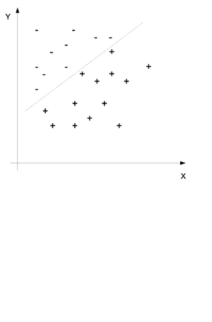
We would like to obtain the probability distribution of the following equation where c is the class and x and y are the data points. In simple terms we would like to find the probability that this point is in class c when we know that the values of x and Y are x and y.
Clustering
Clustering is unsupervised learning method that assign different a set of data point into a group or cluster based on the similarity between the data points. Clustering is somehow like classification only that we do not know the groups before we gather and examine the data. We would like to find the probability distribution of the following equation without knowing the value of c.
Density Estimation
Density Estimation is the problem of modeling a probability density function p(x), given a finite number of data points drawn from that density function.
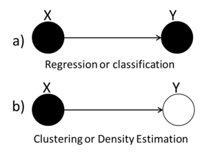
We can use graphs to represent the four types of statistical problems that have been introduced so far. The first graph (Fig.36(a)) can be used to represent either the Regression or the Classification problem because both the X and the Y variables are known. The second graph (Fig.36(b)) we see that the value of the Y variable is unknown and so we can tell that this graph represents the Clustering and Density Estimation situation.
Likelihood Function
Recall that the probability model [math]\displaystyle{ p(x|\theta) }[/math] has the intuitive interpretation of assigning probability to X for each fixed value of [math]\displaystyle{ \theta }[/math]. In the Bayesian approach this intuition is formalized by treating [math]\displaystyle{ p(x|\theta) }[/math] as a conditional probability distribution. In the Frequentist approach, however, we treat [math]\displaystyle{ p(x|\theta) }[/math] as a function of [math]\displaystyle{ \theta }[/math] for fixed x, and refer to [math]\displaystyle{ p(x|\theta) }[/math] as the likelihood function.
where [math]\displaystyle{ p(x|\theta) }[/math] is the likelihood L([math]\displaystyle{ \theta, x }[/math])
where [math]\displaystyle{ log(p(x|\theta)) }[/math] is the log likelihood [math]\displaystyle{ l(\theta, x) }[/math]
Since [math]\displaystyle{ p(x) }[/math] in the denominator of Bayes Rule is independent of [math]\displaystyle{ \theta }[/math] we can consider it as a constant and we can draw the conclusion that:
Symbolically, we can interpret this as follows:
where we see that in the Bayesian approach the likelihood can be viewed as a data-dependent operator that transforms between the prior probability and the posterior probability.
Maximum likelihood
The idea of estimating the maximum is to find the optimum values for the parameters by maximizing a likelihood function form the training data. Suppose in particular that we force the Bayesian to choose a particular value of [math]\displaystyle{ \theta }[/math]; that is, to remove the posterior distribution [math]\displaystyle{ p(\theta|x) }[/math] to a point estimate. Various possibilities present themselves; in particular one could choose the mean of the posterior distribution or perhaps the mode.
(i) the mean of the posterior (expectation):
is called Bayes estimate.
OR
(ii) the mode of posterior:
Note that MAP is Maximum a posterior.
When the prior probabilities, [math]\displaystyle{ p(\theta) }[/math] is taken to be uniform on [math]\displaystyle{ \theta }[/math], the MAP estimate reduces to the maximum likelihood estimate, [math]\displaystyle{ \hat{\theta}_{ML} }[/math].
When the prior is not taken to be uniform, the MAP estimate will be the maximization over probability distributions(the fact that the logarithm is a monotonic function implies that it does not alter the optimizing value).
Thus, one has:
as an alternative expression for the MAP estimate.
Here, [math]\displaystyle{ log (p(x|\theta)) }[/math] is log likelihood and the "penalty" is the additive term [math]\displaystyle{ log(p(\theta)) }[/math]. Penalized log likelihoods are widely used in Frequentist statistics to improve on maximum likelihood estimates in small sample settings.
Example : Bernoulli trials
Consider the simple experiment where a biased coin is tossed four times. Suppose now that we also have some data [math]\displaystyle{ D }[/math]:
e.g. [math]\displaystyle{ D = \left\lbrace h,h,h,t\right\rbrace }[/math]. We want to use this data to estimate [math]\displaystyle{ \theta }[/math]. The probability of observing head is [math]\displaystyle{ p(H)= \theta }[/math] and the probability of observing a tail is [math]\displaystyle{ p(T)= 1-\theta }[/math].
where the conditional probability is
We would now like to use the ML technique.Since all of the variables are iid then there are no dependencies between the variables and so we have no edges from one node to another.
How do we find the joint probability distribution function for these variables? Well since they are all independent we can just multiply the marginal probabilities and we get the joint probability.
This is in fact the likelihood that we want to work with. Now let us try to maximise it:
Take the derivative and set it to zero:
Where:
NH = number of all the observed of heads

NT = number of all the observed tails

Hence, [math]\displaystyle{ NT + NH = n }[/math]
And now we can solve for [math]\displaystyle{ \theta }[/math]:
Example : Multinomial trials
Recall from the previous example that a Bernoulli trial has only two outcomes (e.g. Head/Tail, Failure/Success,…). A Multinomial trial is a multivariate generalization of the Bernoulli trial with K number of possible outcomes, where K > 2. Let [math]\displaystyle{ p(k) = \theta_k }[/math] be the probability of outcome k. All the [math]\displaystyle{ \theta_k }[/math] parameters must be:
[math]\displaystyle{ 0 \leq \theta_k \leq 1 }[/math]
and
[math]\displaystyle{ \sum_k \theta_k = 1 }[/math]
Consider the example of rolling a die M times and recording the number of times each of the six die's faces observed. Let [math]\displaystyle{ N_k }[/math] be the number of times that face k was observed.
Let [math]\displaystyle{ [x^m = k] }[/math] be a binary indicator, such that the whole term would equals one if [math]\displaystyle{ x^m = k }[/math], and zero otherwise. The likelihood function for the Multinomial distribution is:
[math]\displaystyle{ l(\theta; D) = log( p(D|\theta) ) }[/math]
[math]\displaystyle{ = log(\prod_m \theta_{x^m}^{x}) }[/math]
[math]\displaystyle{ = log(\prod_m \theta_{1}^{[x^m = 1]} ... \theta_{k}^{[x^m = k]}) }[/math]
[math]\displaystyle{ = \sum_k log(\theta_k) \sum_m [x^m = k] }[/math]
[math]\displaystyle{ = \sum_k N_k log(\theta_k) }[/math]
Take the derivatives and set it to zero:
[math]\displaystyle{ \frac{\partial l}{\partial\theta_k} = 0 }[/math]
[math]\displaystyle{ \frac{\partial l}{\partial\theta_k} = \frac{N_k}{\theta_k} - M = 0 }[/math]
[math]\displaystyle{ \Rightarrow \theta_k = \frac{N_k}{M} }[/math]
Example: Univariate Normal
Now let us assume that the observed values come from normal distribution.
\includegraphics{images/fig4Feb6.eps}
\newline
Our new model looks like:
Now to find the likelihood we once again multiply the independent marginal probabilities to obtain the joint probability and the likelihood function.
Now, since our parameter theta is in fact a set of two parameters,
we must estimate each of the parameters separately.
Discriminative vs Generative Models
(beginning of Oct. 18) If we call the evidence/features variable [math]\displaystyle{ X\,\! }[/math] and the output variable [math]\displaystyle{ Y\,\! }[/math], one way to model a classifier is to base the definition of the joint distribution on [math]\displaystyle{ p(X|Y)\,\! }[/math] and another one is to do it based on [math]\displaystyle{ p(Y|X)\,\! }[/math]. The first of this two approaches is called generative, as the second one is called discriminative. The philosophy behind this naming might be clear by looking at the way each conditional probability function tries to present a model. Based on the experience, using generative models (e.g. Bayes Classifier) in many cases leads to taking some assumptions which may not be valid according to the nature of the problem and hence make a model depart from the primary intentions of a design. This may not be the case for discriminative models (e.g. Logistic Regression), as they do not depend on many assumptions besides the given data.
Markov Models
Markov models, introduced by Andrey (Andrei) Andreyevich Markov as a way of modeling Russian peotry, are known as a good way of modeling those processes which progress over time or space. Basically, a Markov model can be formulated as follows:
Which can be interpreted by the dependence of the current state of a variable on its last [math]\displaystyle{ k }[/math] states. (Fig. XX)
Maximum Entropy Markov model is a type of Markov model, which makes the current state of a variable dependant on some global variables, besides the local dependencies. As an example, we can define the sequence of words in a context as a local variable, as the appearance of each word depends mostly on the words that have came before (n-grams). However, the role of POS (part of speech tagging) can not be denied, as it affect the sequence of words very clearly. In this example, POS are global dependencies, whereas last words in a row are those of local.
Graph Structure
Up to this point, we have covered many topics about graphical models, assuming that the graph structure is given. However, finding an optimal structure for a graphical model is a challenging problem all by itself. In this section, we assume that the graphical model that we are looking for is expressible in a form of tree. And to remind ourselves of the concept of tree, an undirected graph will be a tree, if there is one and only one path between each pair of nodes. For the case of directed graphs, however, on top of the mentioned condition, we also need to check if all the nodes have at most one parent - which is in other words no explaining away kinds of structures.
Firstly, let us show you how it does not affect the joint distribution function, if a graph is directed or undirected, as long as it is tree. Here is how one can write down the joint ditribution of the graph of Fig. XX.
Now, if we change the direction of the connecting edge between [math]\displaystyle{ x_1 }[/math] and [math]\displaystyle{ x_2 }[/math], we will have the graph of Fig. XX and the corresponding joint distribution function will change as follows:
which can be simply re-written as:
which is the same as the first function. We will depend on this very simplistic observation and leave the proof to the enthusiast reader.
Maximum Likelihood Tree
Optimality of a tree structure can be discussed in terms of likelihood of the set of variables. By doing so, we can define a fully connected, weighted graph by setting the edge weights to the likelihood of the occurrence of the connecting nodes/random variables and then by running the maximum weight spanning tree. Here is how it works.
We have defined the joint distribution as follows:
Where [math]\displaystyle{ V }[/math] and [math]\displaystyle{ E }[/math] are respectively the sets of vertices and edges of the corresponding graph. This holds as long as the tree structure for the graphical model is concerned, as the dependence of [math]\displaystyle{ x_i }[/math] on [math]\displaystyle{ x_j }[/math] has been chosen arbitrarily and this is not the case for non-tree graphical models.
Maximizing the joint probability distribution over the given set of data samples [math]\displaystyle{ X }[/math] with the objective of parameter estimation we will have (MLE):
And by taking the logarithm of [math]\displaystyle{ L(\theta|X) }[/math] (log-likelihood), we will get:
As much as the optimization of the tree structure is concerned, the probability of the single nodes may not play any role in the optimization, so we can define the cost function for our optimization problem as such:
Where the sub r is for reduced. By replacing the probability functions with the frequency of occurence of each state, we will have:
Where we have assumed that [math]\displaystyle{ p(x_i,x_j)=\frac{N_{ijst}}{N} }[/math], [math]\displaystyle{ p(x_i)=\frac{N_{is}}{N} }[/math], and [math]\displaystyle{ p(x_j)=\frac{N_{jt}}{N} }[/math]. The resulting statement is the definition of the mutual information of the two random variables [math]\displaystyle{ x_i }[/math] and [math]\displaystyle{ x_j }[/math], where the former is in state [math]\displaystyle{ s }[/math] and the latter in [math]\displaystyle{ t }[/math].
This is how it has been figured out how to define weights for the edges of a fully connected graph. Now, it is required to run the maximum weight spanning tree on the resulting graph to find the optimal structure for the tree. It is important to note that before developing graphical models this problem has been solved in graph theory. Here our problem was completely a probabilistic problem but using graphical models we could find an equivalent graph theory problem. This show how graphical models can help us to use powerful graph theory tools to solve probabilistic problems.
Latent Variable Models
(beginning of Oct. 20) Assuming that we have thoroughly observed, or even identified all of the random variables of a model can be a very naive assumption, as one can think of many instances of contrary cases. To make a model as rich as possible -there is always a trade-off between richness and complexity, so we do not like to inject unnecessary complexity to our model either- the concept of latent variables has been introduced to the graphical models.
Depending on the position of an unobserved variable, [math]\displaystyle{ z }[/math], we take different actions. If there is no variable conditioned on [math]\displaystyle{ z }[/math], we can integrate/sum it out and it will never be noticed, as it is not either an evidence or a querey. However, we will require to model an unobserved variable like [math]\displaystyle{ z }[/math], if it is bound to some conditions.
The use of latent variables makes a model harder to analyze and to learn. The use of log-likelihood used to make the target function easier to obtain, as the log of product will change to sum of logs, but this will not be the case, when one introduces latent variables to a model, as the resulting joint probability function comes with a sum, which makes the effect of log on product impossible.
As an example of latent variables, one can think of a mixture density model. There are different models come together to build the final model, but it takes one more random variable to say which one of those models to use at the presence of each new sample point. This will affect both the learning and recalling phases.
Appendix: Graph Drawing Tools
Graphviz
"Graphviz is open source graph visualization software. Graph visualization is a way of representing structural information as diagrams of abstract graphs and networks. It has important applications in networking, bioinformatics, software engineering, database and web design, machine learning, and in visual interfaces for other technical domains." <ref>http://www.graphviz.org/</ref>
AISee
AISee is a commercial graph visualization software. The free trial version has almost all the features of the full version except that it should not be used for commercial purposes.
TikZ
"TikZ and PGF are TeX packages for creating graphics programmatically. TikZ is build on top of PGF and allows you to create sophisticated graphics in a rather intuitive and easy manner." <ref> http://www.texample.net/tikz/ </ref>
Xfig
"Xfig" is an open source drawing software used to create objects of various geometry. It can be installed on both windows and unix based machines. Website