stat940F24

Regularization in Deep Learning

Introduction

Regularization is a fundamental concept in machine learning, particularly in deep learning, where models with a high number of parameters are prone to overfitting. Overfitting occurs when a model learns the noise in the training data rather than the underlying distribution, leading to poor generalization on unseen data. Regularization techniques aim to constrain the model’s capacity, thus preventing overfitting and improving generalization. This chapter will explore various regularization methods in detail, complete with mathematical formulations, intuitive explanations, and practical implementations.

L2 Parameter Regularization (Weight Decay)

Overview

L2 parameter regularization, commonly known as weight decay, is a technique used to prevent overfitting in machine learning models by penalizing large weights. This penalty helps in constraining the model's complexity.

The regularization term is given by:

[math]\displaystyle{ \mathcal{R}(w) = \frac{\lambda}{2} \|w\|_2^2 }[/math]

where:

• [math]\displaystyle{ \lambda }[/math] is the regularization strength (a hyperparameter),
• [math]\displaystyle{ w }[/math] represents the model weights,
• [math]\displaystyle{ \|w\|_2 }[/math] denotes the L2 norm of the weight vector.

Gradient of the Total Objective Function

The gradient of the total objective function, which includes both the loss and the regularization term, is given by:

[math]\displaystyle{ \nabla_w \mathcal{L}_{\text{total}}(w; X, y) = \lambda w + \nabla_w \mathcal{L}(w; X, y) }[/math]

The weight update rule with L2 regularization using gradient descent is:

[math]\displaystyle{ w := w - \eta (\lambda w + \nabla_w \mathcal{L}(w; X, y)) }[/math]

where [math]\displaystyle{ \eta }[/math] is the learning rate.

Quadratic Approximation to the Objective Function

Consider a quadratic approximation to the objective function:

[math]\displaystyle{ \mathcal{L}(w) \approx \mathcal{L}(w^*) + \frac{1}{2} (w - w^*)^\top H (w - w^*) }[/math]

where:

• [math]\displaystyle{ w^* }[/math] is the optimum weight vector,
• [math]\displaystyle{ H }[/math] is the Hessian matrix of second derivatives.

The modified gradient equation becomes:

[math]\displaystyle{ \lambda w + H (w - w^*) = 0 }[/math]

Solving for [math]\displaystyle{ w }[/math], we get:

[math]\displaystyle{ w = (H + \lambda I)^{-1} H w^* }[/math]

where [math]\displaystyle{ I }[/math] is the identity matrix.

Eigenvalue Decomposition

Assume [math]\displaystyle{ H = Q \Lambda Q^\top }[/math] where [math]\displaystyle{ Q }[/math] is the orthogonal matrix of eigenvectors and [math]\displaystyle{ \Lambda }[/math] is the diagonal matrix of eigenvalues.

Then the weight vector can be expressed as:

[math]\displaystyle{ w = Q(\Lambda + \lambda I)^{-1} \Lambda Q^\top w^* }[/math]

The effect of weight decay is to rescale the coefficients of the eigenvectors. The [math]\displaystyle{ i }[/math]-th component is rescaled by a factor of [math]\displaystyle{ \frac{\lambda_i}{\lambda_i + \lambda} }[/math], where [math]\displaystyle{ \lambda_i }[/math] is the [math]\displaystyle{ i }[/math]-th eigenvalue.

• If [math]\displaystyle{ \lambda_i \gt \lambda }[/math], the effect of regularization is relatively small.
• Components with [math]\displaystyle{ \lambda_i \lt \lambda }[/math] will be shrunk to have nearly zero magnitude.

Effective Number of Parameters

Directions along which the parameters contribute significantly to reducing the objective function are preserved. A small eigenvalue of the Hessian indicates that movement in this direction will not significantly increase the gradient.

The effective number of parameters can be defined as:

[math]\displaystyle{ \text{Effective Number of Parameters} = \sum_i \frac{\lambda_i}{\lambda_i + \lambda} }[/math]

As [math]\displaystyle{ \lambda }[/math] increases, the effective number of parameters decreases, which reduces the model's complexity.

(Placeholder for Image) (Include an image illustrating the effect of weight decay on the eigenvalues and the effective number of parameters)

Dataset Augmentation

Overview

Dataset augmentation is a technique used to improve the generalization ability of machine learning models by artificially increasing the size of the training dataset. This is particularly useful when the amount of available data is limited. The idea is to create new, synthetic data by applying various transformations to the original dataset.

• Key Idea: The best way to make a machine learning model generalize better is to train it on more data. When the amount of available data is limited, creating synthetic data (e.g., by applying transformations like rotation, translation, and noise addition) and adding it to the training set can be effective.

• Practical Example: Operations like translating training images a few pixels in each direction can greatly improve generalization. Another approach is to train neural networks with random noise applied to their inputs, which also serves as a form of dataset augmentation. This technique can be applied not only to the input layer but also to hidden layers, effectively performing dataset augmentation at multiple levels of abstraction.

---

Noise Injection

Overview

Noise injection is a regularization strategy that can be applied in two main ways:

1. Adding Noise to the Input: This method can be interpreted as a form of dataset augmentation and also has a direct connection to traditional regularization methods. 2. Adding Noise to the Weights: This method is primarily used in the context of recurrent neural networks and can be viewed as a stochastic implementation of Bayesian inference over the weights.

Mathematical Proof for Injecting Noise at the Input

Consider a regression setting where we have an input-output pair \( (x, y) \) and the goal is to minimize the expected loss function:

[math]\displaystyle{ J = \mathbb{E}_{x, y} \left[(f(x) - y)^2\right] }[/math]

Now, suppose we inject noise into the input \( x \), where the noise \( \epsilon \) is drawn from a distribution with mean zero (e.g., Gaussian noise \( \epsilon \sim \mathcal{N}(0, \sigma^2) \)). The modified objective function with noise-injected inputs becomes:

[math]\displaystyle{ J_{\text{noise}} = \mathbb{E}_{x, y, \epsilon} \left[(f(x + \epsilon) - y)^2\right] }[/math]

To understand the effect of noise injection, we can expand the function \( f(x + \epsilon) \) around \( x \) using a Taylor series:

[math]\displaystyle{ f(x + \epsilon) = f(x) + \epsilon^\top \nabla_x f(x) + \frac{1}{2} \epsilon^\top \nabla_x^2 f(x) \epsilon + \mathcal{O}(\|\epsilon\|^3) }[/math]

Since the expectation of the noise \( \epsilon \) is zero:

[math]\displaystyle{ \mathbb{E}[\epsilon] = 0 }[/math]

and assuming that the noise is isotropic with covariance matrix \( \sigma^2 I \), the expectation of the second-order term becomes:

[math]\displaystyle{ \mathbb{E}[\epsilon \epsilon^\top] = \sigma^2 I }[/math]

Substituting the Taylor expansion into the objective function:

[math]\displaystyle{ J_{\text{noise}} = \mathbb{E}_{x, y} \left[(f(x) - y)^2\right] + \frac{\sigma^2}{2} \mathbb{E}_{x, y} \left[\|\nabla_x f(x)\|^2\right] + \mathcal{O}(\sigma^4) }[/math]

This shows that the objective function with noise injection is equivalent to the original objective function plus a regularization term that penalizes large gradients of the function \( f(x) \). Specifically, the added term [math]\displaystyle{ \frac{\sigma^2}{2} \mathbb{E}_{x, y} \left[\|\nabla_x f(x)\|^2\right] }[/math] reduces the sensitivity of the network's output to small variations in its input.

Key Result:

For small noise variance \( \sigma^2 \), the minimization of the loss function with noise-injected input is equivalent to minimizing the original loss function with an additional regularization term that penalizes large gradients:

[math]\displaystyle{ J_{\text{noise}} \approx J + \frac{\sigma^2}{2} \mathbb{E}_{x, y} \left[\|\nabla_x f(x)\|^2\right] }[/math]

This regularization term effectively reduces the sensitivity of the output with respect to small changes in the input \( x \), which is beneficial in avoiding overfitting.

Connection to Weight Decay:

In linear models, where \( f(x) = w^\top x \), the gradient \( \nabla_x f(x) \) is simply the weight vector \( w \). Therefore, the regularization term becomes:

[math]\displaystyle{ \frac{\sigma^2}{2} \|w\|^2 }[/math]

which is equivalent to L2 regularization or weight decay.

Manifold Tangent Classifier

Overview

The Manifold Tangent Classifier (MTC) is a classification technique that leverages the idea that data often lies on a lower-dimensional manifold within the high-dimensional input space. The key assumption is that examples on the same manifold share the same category, and the classifier should be invariant to local factors of variation that correspond to movements on the manifold.

• Key Idea: The classifier should be invariant to variations along the manifold while being sensitive to changes that move the data off the manifold.

Tangent Propagation Algorithm

One approach to achieve invariance to manifold variations is to use the Tangent-Prop algorithm (Simard et al., 1992). The main idea is to add a penalty to the loss function that encourages the neural network's output to be locally invariant to known factors of variation. This is achieved by requiring the gradient of the output with respect to the input to be orthogonal to the known manifold tangent vectors \( v_i \) at each point \( x \).

The regularization term can be expressed as:

[math]\displaystyle{ \text{Regularizer} = \lambda \sum_{i} \left(\frac{\partial f(x)}{\partial x} \cdot v_i \right)^2 }[/math]

where:

• \( \frac{\partial f(x)}{\partial x} \) is the gradient of the neural network output with respect to the input,
• \( v_i \) are the known tangent vectors of the manifold,
• \( \lambda \) is the regularization strength.

This regularization ensures that the directional derivative of \( f(x) \) in the directions \( v_i \) is small, promoting invariance along the manifold.

Manifold Tangent Classifier (MTC)

A more recent approach, introduced by Rifai et al. (2011), eliminates the need to know the tangent vectors a priori. The Manifold Tangent Classifier automatically learns these tangent vectors during training, making it more flexible and applicable to a wider range of problems.

---

Early Stopping as a Form of Regularization

Overview

Early stopping is one of the most commonly used forms of regularization in deep learning. Instead of running the optimization algorithm until it reaches a local minimum of the training error, early stopping involves monitoring the validation error during training and halting the process when the validation error stops improving.

• Key Idea: During training, whenever the error on the validation set improves, a copy of the model parameters is stored. The training is stopped when the validation error has not improved for a predetermined amount of time, and the best model parameters (those that resulted in the lowest validation error) are returned.

Mathematical Formulation

Assume that \( w \) represents the model weights (ignoring bias parameters). We take a quadratic approximation to the objective function \( J(w) \) around the empirically optimal value of the weights \( w^* \):

[math]\displaystyle{ J(w) \approx J(w^*) + \frac{1}{2} (w - w^*)^\top H (w - w^*) }[/math]

where:

• \( H \) is the Hessian matrix of second derivatives.

The gradient of the objective function is:

[math]\displaystyle{ \nabla_w J(w) = H(w - w^*) }[/math]

During training, the parameter vector is updated according to:

[math]\displaystyle{ w^{(t+1)} = w^{(t)} - \eta \nabla_w J(w^{(t)}) }[/math]

Substituting the expression for the gradient:

[math]\displaystyle{ w^{(t+1)} - w^* = (I - \eta H) (w^{(t)} - w^*) }[/math]

where \( \eta \) is the learning rate. If we assume that the initial weights are zero (i.e., \( w^{(0)} = 0 \)), we can express the weight update after \( t \) iterations as:

[math]\displaystyle{ w^{(t)} - w^* = (I - \eta H)^t (w^{(0)} - w^*) }[/math]

If we perform an eigenvalue decomposition of \( H \), we get:

[math]\displaystyle{ H = Q \Lambda Q^\top }[/math]

where \( Q \) is the orthogonal matrix of eigenvectors, and \( \Lambda \) is the diagonal matrix of eigenvalues. The weight update can then be rewritten as:

[math]\displaystyle{ w^{(t)} - w^* = Q (I - \eta \Lambda)^t Q^\top (w^{(0)} - w^*) }[/math]

Assuming \( w^{(0)} = 0 \) and that \( |1 - \eta \lambda_i| < 1 \) for all eigenvalues \( \lambda_i \), after \( t \) training updates, we have:

[math]\displaystyle{ Q^\top w^{(t)} \approx [I - (1 - \eta \Lambda)^t] Q^\top w^* }[/math]

Taking the logarithm and using the series expansion for \( \log(1 + x) \), it can be shown that the number of training iterations \( t \) plays a role inversely proportional to the L2 regularization parameter \( \lambda \), and the inverse of \( t \) plays the role of the weight decay coefficient.

Key Insight:

This result shows that early stopping can be interpreted as a form of implicit regularization, where the number of training iterations controls the effective complexity of the model.

Early Stopping as a Form of Regularization

Overview

Early stopping is one of the most commonly used forms of regularization in deep learning. Instead of running the optimization algorithm until it reaches a local minimum of the training error, early stopping involves monitoring the validation error during training and halting the process when the validation error stops improving.

• Key Idea: During training, whenever the error on the validation set improves, a copy of the model parameters is stored. The training is stopped when the validation error has not improved for a predetermined amount of time, and the best model parameters (those that resulted in the lowest validation error) are returned.

Mathematical Formulation

Assume that \( w \) represents the model weights (ignoring bias parameters). We take a quadratic approximation to the objective function \( J(w) \) around the empirically optimal value of the weights \( w^* \):

[math]\displaystyle{ J(w) \approx J(w^*) + \frac{1}{2} (w - w^*)^\top H (w - w^*) }[/math]

where:

\( H \) is the Hessian matrix of second derivatives.

The gradient of the objective function is:

[math]\displaystyle{ \nabla_w J(w) = H(w - w^*) }[/math]

During training, the parameter vector is updated according to:

[math]\displaystyle{ w^{(t+1)} = w^{(t)} - \eta \nabla_w J(w^{(t)}) }[/math]

Substituting the expression for the gradient:

[math]\displaystyle{ w^{(t+1)} - w^* = (I - \eta H) (w^{(t)} - w^*) }[/math]

where \( \eta \) is the learning rate. If we assume that the initial weights are zero (i.e., \( w^{(0)} = 0 \)), we can express the weight update after \( t \) iterations as:

[math]\displaystyle{ w^{(t)} - w^* = (I - \eta H)^t (w^{(0)} - w^*) }[/math]

If we perform an eigenvalue decomposition of \( H \), we get:

[math]\displaystyle{ H = Q \Lambda Q^\top }[/math]

where \( Q \) is the orthogonal matrix of eigenvectors, and \( \Lambda \) is the diagonal matrix of eigenvalues. The weight update can then be rewritten as:

[math]\displaystyle{ w^{(t)} - w^* = Q (I - \eta \Lambda)^t Q^\top (w^{(0)} - w^*) }[/math]

Assuming \( w^{(0)} = 0 \) and that \( |1 - \eta \lambda_i| < 1 \) for all eigenvalues \( \lambda_i \), after \( t \) training updates, we have:

[math]\displaystyle{ Q^\top w^{(t)} \approx [I - (1 - \eta \Lambda)^t] Q^\top w^* }[/math]

Taking the logarithm and using the series expansion for \( \log(1 + x) \), it can be shown that the number of training iterations \( t \) plays a role inversely proportional to the L2 regularization parameter \( \lambda \), and the inverse of \( t \) plays the role of the weight decay coefficient.

Key Insight:

This result shows that early stopping can be interpreted as a form of implicit regularization, where the number of training iterations controls the effective complexity of the model.

Label Smoothing

Label smoothing is a technique to prevent a model from becoming over-confident on a specific class by not forcing the model to fit the data exactly. This approach provides more flexibility and generalization abilities.

Suppose the predicted output is [math]\displaystyle{ y = [0, 1, 0] }[/math], then after applying label smoothing, it becomes [math]\displaystyle{ y = [0.033, 0.933, 0.033] }[/math].

The formula for label smoothing is:

[math]\displaystyle{ y_{\text{smooth}} = (1 - a) \cdot y + \frac{a}{k} }[/math]

where:

• [math]\displaystyle{ a }[/math] is the smoothing factor,
• [math]\displaystyle{ y }[/math] is the original label,
• [math]\displaystyle{ k }[/math] is the number of classes.

The reason for using label smoothing:

• Prevents overfitting: By preventing the model from becoming too confident in its predictions, label smoothing reduces the likelihood of overfitting.
• Improves generalization: Label smoothing can help the model generalize better to unseen data, as it discourages overconfidence in training.

Bagging/Ensemble

Bagging (short for bootstrap aggregating) is a machine learning ensemble technique for reducing generalization error by combining several models (Breiman, 1994)

Explanation: Aggregating is to ombine the predictions of each model, often using voting (for classification) or averaging (for regression).

It works by training several different models separately, and then have all of the models vote on the output for test examples. For example, random forest, which is a popular bagging algorithm that builds multiple decision trees on different bootstrap samples of the data and aggregates their predictions.

The reason why bagging works:

• Variance reduction: By training multiple models on different data subsets, bagging reduces the variance of the predictions. This means that it helps models generalize better to new, unseen data.
• Handling overfitting: Bagging is particularly useful for high-variance models (e.g., decision trees) as it helps reduce overfitting.

While bagging is highly useful for traditional machine learning models, it is less commonly used in deep learning because modern neural networks are already highly expressive. Instead, other ensemble methods, such as model ensembling or dropout, are used.

Code Sample:

from sklearn.ensemble import RandomForestClassifier

from sklearn.datasets import load_iris

from sklearn.model_selection import train_test_split

- Load a dataset (Iris dataset for example) data = load_iris()

X_train, X_test, y_train, y_test = train_test_split(data.data, data.target, test_size=0.3, random_state=42)

- Train a random forest classifier (bagging technique)

rf_model = RandomForestClassifier(n_estimators=100, random_state=42)

rf_model.fit(X_train, y_train)

- Make predictions

y_pred = rf_model.predict(X_test)

- Evaluate the model

accuracy = rf_model.score(X_test, y_test)

Dropout

Overview

Dropout is one of the techniques for preventing overfitting in deepneural network which contains a large number of parameters.

The key idea is to randomly drop units from the neural networkduring training.

• During training, dropout samples from number of different “thinned” network.
• At test time, we approximate the effect of averaging the predictions of all these thinned networks

Model

Consider a neural network with [math]\displaystyle{ L }[/math] hidden layers:

• Let [math]\displaystyle{ z^{(l)} }[/math] denote the vector inputs into layer [math]\displaystyle{ l }[/math].
• Let [math]\displaystyle{ y^{(l)} }[/math] denote the vector of outputs from layer [math]\displaystyle{ l }[/math].
• Let [math]\displaystyle{ W^{(l)} }[/math] and [math]\displaystyle{ b^{(l)} }[/math] represent the weights and biases at layer [math]\displaystyle{ l }[/math].

With dropout, the feed-forward operation becomes:

[math]\displaystyle{ r^{(l)} \sim \text{Bernoulli}(p) }[/math]

[math]\displaystyle{ y^{(l)} = r^{(l)} \odot y^{(l)} }[/math]

where [math]\displaystyle{ \odot }[/math] denotes element-wise multiplication.

The feed-forward equation for layer [math]\displaystyle{ l+1 }[/math] becomes:

[math]\displaystyle{ z^{(l+1)} = W^{(l+1)} y^{(l)} + b^{(l+1)} }[/math]

[math]\displaystyle{ y^{(l+1)} = f(z^{(l+1)}) }[/math]

where [math]\displaystyle{ f }[/math] is the activation function.

For any layer [math]\displaystyle{ l }[/math], [math]\displaystyle{ r^{(l)} }[/math] is a vector of independent Bernoulli random variables, each of which has a probability [math]\displaystyle{ p }[/math] of being 1. The vector [math]\displaystyle{ y^{(l)} }[/math] is the input after some hidden units are dropped. The rest of the model remains the same as a regular feed-forward neural network.

Training

Dropout neural network can be trained using stochastic gradientdescent. The only difference here is that we only back propagate on eachthinned network. The gradient for each parameter are averaged over the training cases in each mini-batch.

Test Time

Use a single neural net without dropout If a unit is retained with probability p during training, the outgoing weights of that unit are multiplied by p at test time. [math]\displaystyle{ p \cdot w }[/math]

Additional Regularization

L1 norm

L1 norm regularization, also known as Lasso, is a technique that adds a penalty equal to the absolute value of the magnitude of coefficients to the loss function. This encourages sparsity in the learned weights, meaning it forces some of the weights to become exactly zero, effectively selecting important features and reducing model complexity.

Mixup

Mixup is a data augmentation technique that creates new training examples by taking convex combinations of pairs of input data and their labels. By blending images and labels together, the model learns smoother decision boundaries and becomes more robust to adversarial examples and noise.

Cutout

Cutout is a form of data augmentation where random square regions are masked out (set to zero) in input images during training. This forces the model to focus on a broader range of features across the image rather than relying on any single part, leading to better generalization and robustness.

Gradient Clipping

Gradient clipping is a technique used to prevent the gradients from becoming too large during training, which can cause the model to diverge. This is done by capping the gradients at a predefined threshold, ensuring that updates remain stable, especially in models like recurrent neural networks (RNNs) where exploding gradients are a common issue.

DropConnect

DropConnect is a variation of Dropout, but instead of dropping neurons, it randomly drops connections (weights) between neurons during training. This prevents the co-adaptation of neurons while allowing individual neurons to contribute to learning.

Data Augmentation (beyond Mixup and Cutout)

• Random Flips and Rotations: Randomly flipping (either vertical or horizontal) or rotating images during training to make the model invariant to certain transformations.
• Color Jittering: Modifying the brightness, contrast, saturation, and hue of images to make the model more robust to variations in color.
• Random Cropping and Scaling: Randomly cropping and scaling images to force the model to learn from different perspectives and contexts within the data.

For PyTorch augmentation, one can refer https://pytorch.org/vision/stable/transforms.html

Generalization Paradox

• Models with many parameters tend to overfit
• However, deep neural network, despite using many parameters, works well with unseen data (look up the Double Descent Curve), the reason remains unknown

This phenomenon is illustrated by the Double Descent Curve, where after reaching a peak in test error (due to overfitting), the error decreases again with further model complexity. The precise reasons remain uncertain, but hypotheses include implicit regularization from optimization methods like SGD, hierarchical feature learning, and the redundancy offered by overparameterization.

Batch Normalization

Overview

Batch normalization is a technique used to improve the training process of deep neural networks by normalizing the inputs of each layer. Despite the initial intuition for the method being somewhat incorrect, it has proven to be highly effective in practice. Batch normalization speeds up convergence, allows for larger learning rates, and makes the model less sensitive to initialization, resulting in more stable and efficient training.

Batch normalization motivated by internal covariate shift (2015 lofee & Szegedy)

Internal Covariance Shift

Batch normalization was originally proposed as a solution to the internal covariance shift problem, where the distribution of inputs to each layer changes during training. This shift complicates training because the model must constantly adapt to new input distributions.

The transformation of layers can be described as:

[math]\displaystyle{ l = F_2(F_1(u, \theta_1), \theta_2) }[/math]

For a mini-batch of activations [math]\displaystyle{ X = \{x_1, x_2, \dots, x_m\} }[/math] from a specific layer, batch normalization proceeds as follows:

1. Compute the mean: [math]\displaystyle{ \mu_B = \frac{1}{m} \sum_{i=1}^{m} x_i }[/math]

2. Compute the variance: [math]\displaystyle{ \sigma_B^2 = \frac{1}{m} \sum_{i=1}^{m} (x_i - \mu_B)^2 }[/math]

3. Normalize the activations: [math]\displaystyle{ \hat{x}_i = \frac{x_i - \mu_B}{\sqrt{\sigma_B^2 + \epsilon}} }[/math]

4. Scale and shift the normalized activations using learned parameters [math]\displaystyle{ \gamma }[/math] (scale) and [math]\displaystyle{ \beta }[/math] (shift): [math]\displaystyle{ y_i = \gamma \hat{x}_i + \beta }[/math]

where:

• [math]\displaystyle{ x_i }[/math] represents the activations in the mini-batch,
• [math]\displaystyle{ \mu_B }[/math] is the mean of the mini-batch,
• [math]\displaystyle{ \sigma_B^2 }[/math] is the variance of the mini-batch,
• [math]\displaystyle{ \epsilon }[/math] is a small constant added for numerical stability,
• [math]\displaystyle{ \hat{x}_i }[/math] is the normalized activation,
• [math]\displaystyle{ \gamma }[/math] and [math]\displaystyle{ \beta }[/math] are learned parameters for scaling and shifting.

The batch normalization improves validation accuracy by removing the dropout and enables higher learning rate

Batch Normalization

As mentioned earlier, the original intuition behind batch normalization was found to be incorrect after further research. A paper by Santurkar, S., Tsipras, D., Ilyas, A., & Madry, A. (NeurIPS 2019) contradicted the original 2015 paper on BatchNorm by highlighting the following points:

• Batch normalization does not fix covariate shift.
• If we fix covariate shift, it doesn't help.
• lf we intentionally increase lCS, it doesn't harm.
• Batch Norm is not the only possible normalization. There are alternatives.

Instead, they argue that Batch normalization works better due to other factors, particularly related to its effect on the optimization process:

1. Reparameterization of the loss function:

• Improved Lipschitzness: Batch normalization improves the Lipschitz continuity of the loss function, meaning that the loss changes at a smaller rate, and the magnitudes of the gradients are smaller. This makes the gradients of the loss more "Lipschitz."
• Better β-smoothness: The loss exhibits significantly better smoothness, which aids in optimization by preventing large, erratic changes in the gradient.

2. Variation of the loss function: BatchNorm reduces the variability of the value of the loss. Consider the variation of the loss function: [math]\displaystyle{ \mathcal{L}(x + \eta \nabla \mathcal{L}(x)) }[/math] where [math]\displaystyle{ \eta \in [0.05, 0.4] }[/math]. A smaller variability of the loss indicates that the steps taken during training are less likely to cause the loss to increase uncontrollably.

3. Gradient predictiveness: BatchNorm enhances the predictiveness of the gradients, meaning the changes in the loss gradient are more stable and predictable. This can be expressed as: [math]\displaystyle{ || \nabla \mathcal{L}(x) - \nabla \mathcal{L}(x + \eta \nabla \mathcal{L}(x)) || }[/math], where [math]\displaystyle{ \eta \in [0.05, 0.4] }[/math]. A good gradient predictiveness implies that the gradient evaluated at a given point remains relevant over longer distances, which allows for larger step sizes during training.

Alternatives to Batch Norm

Weight Normalization: Weight normalization is a technique where the weights, instead of the activations, are normalized. This method reparameterizes the weight vectors to accelerate the training of deep neural networks.

Tim Salimans and Diederik P. Kingma, "Weight Normalization: A Simple Reparameterization to Accelerate Training of Deep Neural Networks," 2016.

ELU (Exponential Linear Unit) and SELU (Scaled Exponential Linear Unit): ELU and SELU are two proposed activation functions that have a decaying slope instead of a sharp saturation. They can be used as alternatives to BatchNorm by providing smoother, non-linear activation without requiring explicit normalization.

Djork-Arné Clevert, Thomas Unterthiner, and Sepp Hochreiter, "Fast and Accurate Deep Network Learning by Exponential Linear Units (ELUs)," In International Conference on Learning Representations (ICLR), 2016. Günter Klambauer, Thomas Unterthiner, Andreas Mayr, and Sepp Hochreiter, "Self-Normalizing Neural Networks," ICLR, 2017.

Convolutional Neural Network (CNN)

Introduction

Convolutional networks are simply neural networks that use convolution instead of general matrix multiplication in at least one of their layers. CNN is mainly used for image processing.

Convolution

In ML, convolution means dot product

[math]\displaystyle{ h = \sigma(\langle x, w\rangle+b) }[/math]

• Same x, different w -- multi-layer perception (MLP)
• Different x, same w -- CNN (weight sharing)

From class, the following operation is called convolution

[math]\displaystyle{ s(t) = \int x(a)w(t-a)ds }[/math]

The convolution operation is typically denoted with an asterisk:

[math]\displaystyle{ s(t) = (x \ast w)(t) }[/math]

Discrete Convolution

If we now assume that x and w are defined only on integer t, we can define the discrete convolution:

[math]\displaystyle{ s[t] = (x \ast w)(t) = \sum_{a=-\infty}^{\infty} x[a] \, w[t-a] }[/math]

[math]\displaystyle{ w[t-a] }[/math] represents the sequence [math]\displaystyle{ w[t] }[/math] shifted by [math]\displaystyle{ a }[/math] units.

In practice

We often use convolutions over more than one axis at a time.

[math]\displaystyle{ s[i,j] = (I * K)[i,j] = \sum_m \sum_n I[m,n] K[i-m, j-n] }[/math]

• Input: usually a multidimensional array of data.

• Kernel: usually a multidimensional array of parameters that should be learned.

We assume that these functions are zero everywhere but the finite set of points for which we store the values.

We can implement the infinite summation as a summation over a finite number of array elements.

Convolution and Cross-Correlation

Convolution is commutative:

[math]\displaystyle{ s[i,j] = (I * K)[i,j] = \sum_m \sum_n I[i-m, j-n] K[m, n] }[/math]

Cross-correlation:

[math]\displaystyle{ s[i,j] = (I * K)[i,j] = \sum_m \sum_n I[i+m, j+n] K[m, n] }[/math]

Many machine learning libraries implement cross-correlation but call it convolution. In the context of backpropagation in neural networks, cross-correlation simplifies the computation of gradients with respect to the input and kernel.

Visualization of Cross-Correlation and Convolution with Matlab (https://www.youtube.com/v/Ma0YONjMZLI)

Image to Convolved Feature

• Kernel\filter size: weight [math]\displaystyle{ \times }[/math] height, e.g. 3 [math]\displaystyle{ \times }[/math] 3 in below example
• Stride: how many pixels to move the filter each time
• Padding: add zeros (or any other value) around the boundary of the input

Example

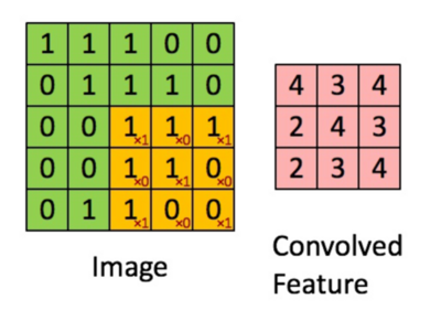
The following image illustrates a 2D convolution operation between an input image and a filter to produce a convolved feature map.

Image (Input): The grid on the left represents a 5[math]\displaystyle{ \times }[/math]5 matrix of pixel values. The orange-highlighted 3[math]\displaystyle{ \times }[/math]3 region is part of the image currently being convolved with the filter.

Convolution Operation: The filter values are applied to the selected region in an element-wise multiplication followed by a summation. The operation is as follows:

[math]\displaystyle{ (1 \times 1) + (1 \times 0) + (1 \times 1) + (0 \times 0) + (1 \times 1) + (1 \times 0) + (0 \times 1) + (0 \times 0) + (1 \times 1) = 4 }[/math]

Convolved Feature Map: The result value [math]\displaystyle{ 4 }[/math], is placed in the corresponding position (top-left) of the convolved feature map on the right.

One Convolution Example

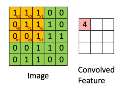
This process is repeated as the filter slides across the entire image. The final feature map is shown below.

Final Feature Map

Sparse Interactions

In feed forward neural network every output unit interacts with every input unit.

• When we have [math]\displaystyle{ m }[/math] inputs and [math]\displaystyle{ n }[/math] outputs, then matrix multiplication requires [math]\displaystyle{ (m \times n) }[/math] parameters. and the algorithms used in practice have [math]\displaystyle{ O(m \times n) }[/math] runtime (per example)

Convolutional networks, typically have sparse connectivity (sparse weights). This is accomplished by making the kernel smaller than the input.

• Limit the number of connections each output may have to [math]\displaystyle{ k }[/math], then requires only [math]\displaystyle{ (k \times n) }[/math] parameters and [math]\displaystyle{ O(k \times n) }[/math] runtime

Parameter Sharing

• In a traditional neural net, each element of the weight matrix is multiplied by one element of the input. i.e. It is used once when computing the output of a layer.
• In CNNs, each member of the kernel is used at every position of the input
• Instead of learning a separate set of parameters for every location, we learn only one set

Equivariance

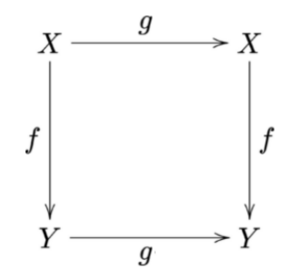
A function [math]\displaystyle{ f(x) }[/math] is equivaraint to a function [math]\displaystyle{ g }[/math] is the following holds:

[math]\displaystyle{ f(g(x)) = g(f(x)) }[/math]

In simple terms: Applying the function [math]\displaystyle{ f }[/math] after [math]\displaystyle{ g }[/math] is equivalent to applying [math]\displaystyle{ g }[/math] after [math]\displaystyle{ f }[/math]

Equivariance

Equivariance in CNNs

• CNNs are naturally equivariant to translation (Covlution = Shift)
• If an input image is shifted, the output feature map shifts correspondingly, preserving spatial structure
• Importance: This property ensures that CNNs can detect features like edges or corners, no matter where they appear in the image

A convolutional layer has equivariance to translation. For example,

[math]\displaystyle{ g(x)[i] = x[i-1] }[/math]

If we apply this transformation to x, then apply convolution, the result will be the same as if we applied convolution to x, then applied the transformation to the output.

For images, convolution creates a 2-D map of where certain features appear in the input. Note that convolution is not equivariant to some other transformations, such as changes in the scale (rescaling) or rotation of an image.

Importance of Data Augmentation

Data augmentation is commonly used to make CNNs robust against variations in scale, rotation, or other transformations. This involves artificially modifying the training data by applying transformations like flipping, scaling, and rotating to expose the network to different variations of the same object.

Convolutional Networks

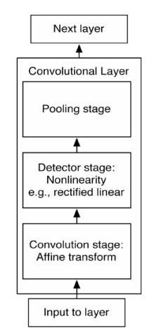
The first stage (Convolution): The layer performs several convolutions in parallel to produce a set of preactivations. The convolution stage is designed to detect local features in the input image, such as edges and patterns. It does this by applying filters/kernels across the input image.

The second stage (Detector): Each preactivation is run through a nonlinear activation function (e.g. rectified linear). This stage introduces nonlinearity into the model, enabling it to learn complex patterns. Without this nonlinearity, the model would be limited to learning only linear relationships.

The third stage (Pooling) Pooling reduces the spatial dimensions of the feature maps (height and width), helping to make the model more invariant to small translations and distortions in the input image. It also reduces computational load and helps prevent overfitting.

CNN Structure

Pooling

Down-sample input size to reduce computation and memory

Popular Pooling functions

• The maximum of a rectangular neighborhood (Max pooling operation)
• The average of a rectangular neighborhood
• The L2 norm of a rectangular neighborhood
• A weighted average based on the distance from the central pixel

Pooling with Downsampling

Max-pooling with a pool width of 3 and a stride between pools of 2. This reduces the representation size by a factor of 2, which reduces the the computational and statistical burden on the next layer.

Pooling and Translations

Pooling helps to make the representation become invariant to small translations of the input. Invariance to local translation can be a very useful property if we care more about whether some feature is present than exactly where it is. For example: In a face, we need not know the exact location of the eyes.

Input of Varying Size

Example: we want to classify images of variable size.

The input to the classification layer must have a fixed size. In the final pooling output (for example) four sets of summary statistics, one for each quadrant of an image, regardless of the image size. Feature after pooling is [math]\displaystyle{ 2 \times 2 }[/math].

It is also possible to dynamically pool features together, for example, by running a clustering algorithm on the locations of interesting features (Boureau et al., 2011).

i.e. a different set of pooling regions for each image.

Learn a single pooling structure that is then applied to all images (Jia et al., 2012)

Convolution and Pooling as an Infinitely Strong Prior

• Weak Prior: a prior distribution that has high entropy, which means there is a high level of uncertainty or spread in the distribution. An example of this would be a Gaussian distribution with high variance
• Strong Prior: has very low entropy, which implies a high level of certainty or concentration in the distribution. An example of this would be a Gaussian distribution with low variance
• Infinitely Strong Prior: places zero probability on some parameters and says a convolutional net is similar to a fully connected net with an infinitely strong prior over its weights

The weights for one hidden unit must be identical to the weights of its neighbor, but shifted in space. The weights must be zero, except for in the small, spatially contiguous receptive field assigned to that hidden unit.

Use of convolution as infinitely strong prior probability distribution over the parameters of a layer. This prior says that the function the layer should learn contains only local interactions and is equivariantto translation.

The use of pooling is infinitely strong prior that each unit should be invariant to small translations. Convolution and pooling can cause underfitting.

Practical Issues

The input is usually not just a grid of real values. It is a grid of vector-valued observations. For example, a color image has a red, green, and blue intensity at each pixel.

When working with images, we usually think of the input and output of the convolution as 3-D tensors. One index into the different channels and two indices into the coordinates of each channel.

Software implementations usually work in batch mode, so they will actually use 4-D tensors, with the fourth axis indexing different examples in the batch.

Training

Suppose we want to train a convolutional network that incorporates convolution of kernel stack [math]\displaystyle{ K }[/math] applied to multi-channel image [math]\displaystyle{ V }[/math] with stride [math]\displaystyle{ s }[/math]:[math]\displaystyle{ c(K; V; s) }[/math]

Suppose we want to minimize some loss function [math]\displaystyle{ J(V; K) }[/math]. During forward propagation, we will need to use [math]\displaystyle{ c }[/math] itself to output [math]\displaystyle{ Z }[/math].

[math]\displaystyle{ Z }[/math] is propagated through the rest of the network and used to compute [math]\displaystyle{ J }[/math].

• During backpropagation, we receive a tensor [math]\displaystyle{ \mathbf{G} }[/math] such that:

[math]\displaystyle{ G_{i,j,k} = \frac{\partial}{\partial Z_{i,j,k}} J(V, K) }[/math]

• To train the network, we compute the derivatives with respect to the weights in the kernel:

[math]\displaystyle{ g(\mathbf{G}, \mathbf{V}, s)_{i,j,k,l} = \frac{\partial}{\partial Z_{i,j,k}} J(V, K) = \sum_{m,n} G_{i,m,n} V_{j,ms+k,ns+l} }[/math]

• If this layer is not the bottom layer of the network, we compute the gradient with respect to [math]\displaystyle{ \mathbf{V} }[/math] to backpropagate the error further:

[math]\displaystyle{ h(\mathbf{K}, \mathbf{G}, s)_{i,j,k} = \frac{\partial}{\partial V_{i,j,k}} J(V, K) = \sum_{l,m \lvert s l + m = j} \sum_{n,p \lvert s n + p = k} \sum_{q} K_{q,i,m,p} G_{i,l,n} }[/math]

Random or Unsupervised Features

The most computationally expensive part of training a convolutional network is learning the features.

• Supervised training with gradient descent requires full forward and backward propagation through the entire network for every gradient update.
• One approach to reduce this cost is to use features that are not learned in a supervised manner, such as random or unsupervised features.

Random Initilizations

Simply initialize the convolution kernels randomly. In high-dimension space, random vectors are almost orthogonal to each other (correlated). Features captured by different kernels are independent.

Unsupervised Learning

Learn the convolution kernels using an unsupervised criterion.

Key insight

Random filters can perform surprisingly well in convolutional networks.

• Layers composed of convolution followed by pooling naturally become frequency-selective and translation-invariant, even with random weights.

Inexpensive architecture selection

• Evaluate multiple convolutional architectures by training only the last layer.
• Choose the best-performing architecture and then fully train it using a more intensive method.

Residual Networks (ResNet)

Overview

Deeper models are harder to train due to vanishing/exploding gradients and can be worse than shallower networks if not properly trained. There are advanced networks to deal with the degradation problem.

ResNet, short for Residual Networks, was introduced by Kaiming He et al. from Microsoft Research in 2015. It brought a significant breakthrough in deep learning by enabling the training of much deeper networks, addressing the vanishing gradient problem.

ResNet Structure

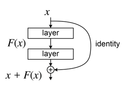
• ResNet introduces the concept of skip connections (or residual connections) that allow the gradient to be directly backpropagated to earlier layers
• Skip connections help in overcoming the degradation problem, where the accuracy saturates and then degrades rapidly as the network depth increases

Variants

Several variants of ResNet have been developed, including ResNet-50, ResNet-101, and ResNet-152, differing in the number of layers.

Application

ResNet has been widely adopted for various computer vision tasks, including image classification, object detection, and facial recognition.

DenseNet

Overview

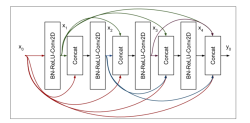
• DenseNet, short for Densely Connected Networks, was introduced by Gao Huang et al. in 2017.
• It is known for its efficient connectivity between layers, which enhances feature propagation and reduces the number of parameters

DenseNet Structure

Key Feature

The key feature is Dense Connectivity.

• In DenseNet, each layer receives feature maps from all preceding layers and passes its own feature maps to all subsequent layers
• This dense connectivity improves the flow of information and gradients throughout the network, mitigating the vanishing gradient problem

Echo State Network

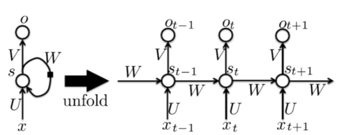
In RNNs, the ability to capture long-term dependencies is crucial. Set the recurrent and input weights such that the recurrent hidden units do a good job of capturing the history of past inputs, and only learn the output weights. The goal is to access the information from the past implicitly.

The hidden state at time [math]\displaystyle{ t }[/math] can be expressed as:

[math]\displaystyle{ s_t = \sigma(W s_{t-1} + U x_t) }[/math]

where:

• [math]\displaystyle{ W }[/math] represents the recurrent weight matrix, which connects previous hidden states to the current state,
• [math]\displaystyle{ U }[/math] is the input weight matrix, responsible for incorporating the current input [math]\displaystyle{ x_t }[/math],
• [math]\displaystyle{ \sigma }[/math] is an activation function, like a non-linear function such as a sigmoid or tanh.

It is important to control how small changes in the hidden state propagate through time to ensure the network does not become unstable.

If a change [math]\displaystyle{ \Delta s }[/math] in the state at time [math]\displaystyle{ t }[/math] is aligned with an eigenvector [math]\displaystyle{ v }[/math] of the Jacobian [math]\displaystyle{ J }[/math] with eigenvalue [math]\displaystyle{ \lambda \gt 1 }[/math], then the small change [math]\displaystyle{ \Delta s }[/math] becomes [math]\displaystyle{ \lambda \Delta s }[/math] after one-time step, and [math]\displaystyle{ \lambda^t \Delta s }[/math] after [math]\displaystyle{ t }[/math] time steps.

If the largest eigenvalue [math]\displaystyle{ \lambda \lt 1 }[/math], the map from [math]\displaystyle{ t }[/math] to [math]\displaystyle{ t+1 }[/math] is contractive.

The network forgets information about the long-term past.

Set the weights to make the Jacobians slightly contractive. This allows the network to gradually forget irrelevant information while still remembering key long-term dependencies.

Echo State Network

Long Delays

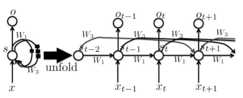
RNNs often fail to capture these dependencies due to the vanishing gradient problem. Long delays use recurrent connections. It knows something from the past, help vanishing gradient - even if gradient get vanished during the path, it still has the direct information from the past.

Long Delays

Leaky Units

In some cases, we do need to forget the path while in some we do not since we do not want to remember redundant information.

Recall that:

[math]\displaystyle{ s_t = \sigma(W s_{t-1} + U x_t) }[/math]

Then consider the following refined form of the equation (convex combination of the current state and previous through a new parameter):

[math]\displaystyle{ s_{t,i} = \left(1 - \frac{1}{\tau_i}\right) s_{t-1} + \frac{1}{\tau_i} \sigma(W s_{t-1} + U x_t) }[/math]

where

• [math]\displaystyle{ 1 \leq \tau_i \leq \infty }[/math]
• [math]\displaystyle{ \tau_i = 1 }[/math] corresponds to an ordinary RNN
• [math]\displaystyle{ \tau_i \gt 1 }[/math] allows gradients to propagate more easily
• [math]\displaystyle{ \tau_i \gg 1 }[/math] means the state changes very slowly, integrating past values associated with the input sequence over a long duration

Infinity means the current state is the previous state while one means completely forgetting the previous steps and only depends on the current observations.

Gated RNNs

Defnition

It might be useful for the neural network to forget the old state in some cases like if we only care about if the current letter is a or b.

Example: [math]\displaystyle{ a\ a\ b\ b\ b\ b\ a\ a\ a\ a\ b\ a\ b }[/math]

It might be useful to keep the memory of the past.

Example:

Instead of manually deciding when to clear the state, we want the neural network to learn to decide when to do it.

Long-Short-Term-Memory (LSTM)

The Long-Short-Term-Memory (LSTM) algorithm was proposed in 1997 (Hochreiter and Schmidhuber, 1997). It is a type of recurrent neural network designed for approaching the vanishing gradient problem.

Several variants of the LSTM are found in the literature:

• Hochreiter and Schmidhuber, 1997
• Graves, 2012
• Graves et al., 2013
• Sutskever et al., 2014

The principle is always to have a linear self-loop through which gradients can flow for a long duration.

Gated Recurrent Units (GRU)

Here is the plain text version of the new image content:

Recent work on gated RNNs, Gated Recurrent Units (GRU), was proposed in 2014.

• Cho et al., 2014
• Chung et al., 2014, 2015
• Jozefowicz et al., 2015
• Chrupala et al., 2015

Standard RNN computes the hidden layer at the next time step directly:

[math]\displaystyle{ s_t = \sigma(W s_{t-1} + U x_t) }[/math]

There are two gates: the update gate and the reset gate. Update gate for the case that we want to keep the information around while reset gate is the case when forgetting. A temporary state locks down some of the values of the current state.

GRU first computes an update gate (another layer) based on the current input vector and hidden state:

[math]\displaystyle{ z_t = \sigma(U^{(z)} x_t + W^{(z)} s_{t-1}) }[/math]

It also computes the reset gate similarly but with different weights:

[math]\displaystyle{ r_t = \sigma(U^{(r)} x_t + W^{(r)} s_{t-1}) }[/math]

New memory content is calculated as:

[math]\displaystyle{ \tilde{s_t} = \tanh(U x_t + r_t \odot W s_{t-1}) }[/math]

which has current observations and forgetting something from the past

If the reset gate is close to 0, this causes the network to ignore the previous hidden state, effectively allowing the model to drop irrelevant information.

The final memory at time step [math]\displaystyle{ t }[/math] is a combination of the current and previous time steps:

[math]\displaystyle{ s_t = z_t \odot s_{t-1} + (1 - z_t) \odot \tilde{s_t} }[/math]

If the reset gate is close to 0, it will ignore the previous hidden state, allowing the model to discard irrelevant information.

The update gate [math]\displaystyle{ z_t }[/math] controls how much of the past state should matter in the current time step. If [math]\displaystyle{ z_t }[/math] is close to 1, then we can effectively copy information from the past state across multiple time steps.

Units that need to capture short-term dependencies often have highly active reset gates.

Cliping Gradients

A simple solution for clipping the gradient. (Mikolov, 2012; Pascanu et al., 2013):

• Clip the parameter gradient from a mini-batch element-wise (Mikolov, 2012) just before the parameter update.
• Clip the norm [math]\displaystyle{ g }[/math] of the gradient [math]\displaystyle{ g }[/math] (Pascanu et al., 2013a) just before the parameter update.

The formula for clipping the gradient is:

[math]\displaystyle{ g' = \min\left(1, \frac{c}{|g|}\right) g }[/math]

Attention

The attention mechanism was introduced to improve the performance of the encoder-decoder model for machine translation.

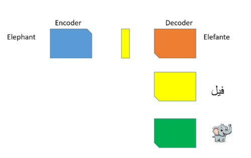
Common Representation

A single 'concept' is universally represented, transcending specific languages or forms.

• Encoder: Processes the word 'elephant' from its original source.
• Output: A universal representation vector (the abstract 'concept' of an elephant).
• Decoders: Translate this concept into various domains or applications.

The 'concept' is an abstract entity that exists independently of any particular language or representation.

For example, if we want to translate from English to Spanish

• Encoder (English Input): The system processes the word "elephant."
• Output (Universal Representation): The system generates an abstract concept or vector representing an "elephant," independent of any specific language.
• Decoder (Spanish Output): The system decodes this concept and outputs the equivalent Spanish word: "elefante."

Common Representation

Sequence-to-Sequence Model

In the sequence-to-sequence model, every word [math]\displaystyle{ x_i }[/math] produces a hidden vector [math]\displaystyle{ h_i }[/math] in the encoder part of the autoencoder. The hidden vector of every word, [math]\displaystyle{ h_i }[/math], is fed to the next hidden vector, [math]\displaystyle{ h_{i+1} }[/math], by a projection matrix [math]\displaystyle{ W }[/math].

In this model, for the whole sequence, there is only one context vector [math]\displaystyle{ c }[/math], which is equal to the last hidden vector of the encoder, i.e., [math]\displaystyle{ c = h_n }[/math].

Sequence-to-Sequence Model

Challenges:

1. Long-range dependencies: As the model processes long sequences, it can struggle to remember and utilize information from earlier steps, especially in cases where long-term context is crucial.

2. Sequential processing: Since these models process data step by step in sequence, they can't take full advantage of parallel processing, which limits the speed and efficiency of training.

These are the core challenges that newer architectures, such as transformers, aim to address.

Attention Definition

The basic idea behind the attention mechanism is directing the focus on important factors when processing data. Attention is a fancy name for weighted average.

Sequence-to-Sequence Model with Attention

• Sequence-to-sequence model:

[math]\displaystyle{ p(y_i | y_1, \ldots, y_{i-1}) = g(y_{i-1}, l_i, c) }[/math]

• Sequence-to-sequence with attention:

[math]\displaystyle{ p(y_i | y_1, \ldots, y_{i-1}) = g(y_{i-1}, l_i, c_i) }[/math]

Sequence-to-Sequence Model with Attention

There are some calculations:

1. Similarity score: [math]\displaystyle{ s_{ij} = similarity(l_{i-1}, h_j) }[/math]

2. Attention weight: [math]\displaystyle{ a_{ij} = \frac{e^{s_{ij}}}{\sum_{k=1}^{T} e^{s_{ik}}} }[/math]

The attention weight [math]\displaystyle{ a_{ij} }[/math] is obtained by applying a softmax function to the similarity scores. This normalizes the scores across all encoder hidden states, turning them into a probability distribution.

3. Context vector: [math]\displaystyle{ c_i = \sum_{j=1}^{T} a_{ij} h_j }[/math]

The effectiveness of the correlation between inputs around position [math]\displaystyle{ j }[/math] and the output at position [math]\displaystyle{ i }[/math] is crucial.

This score is determined based on:

• The RNN hidden state [math]\displaystyle{ l_{i-1} }[/math] just before emitting [math]\displaystyle{ y_i }[/math].
• The [math]\displaystyle{ j^{th} }[/math] hidden state [math]\displaystyle{ h_j }[/math] of the input sentence.

Transformer Architecture

The basic concept behind transformers is attention as summarized in the paper by Vaswani et. al 'Attention is all you need'. Transformer is an example of an encoder-decoder architecture.

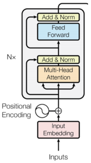
Encoder

The encoder component of transformers consist of two main components: Self Attention and Feed Forward Neural Network. The architecture of the Encoder is given below:

Encoder architecture of the Transformer

Self Attention

Illustration of word2vec where "King" - "Man" + "Woman" produces a vector close to the word "Queen"

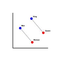
Unlike word2vec introduced in 2013 by Mikolov et al., which captures the vector representations of words in an embedding space such that words that are similar are represented closer to each other, self-attention aims to capture the similarity between words based on context and in relation to each other. For example, the context of the word "bank" differs based on if the surrounding words involve "money" or "river".

Self-attention is analogous to the fundamental retrieval strategy in databases where given a query, and key-value pairs, we use the query to identify the key and retrieve the corresponding value. Given an input vector [math]\displaystyle{ \mathbf{x} \in \mathbb{R}^d }[/math], the weights for the query, key, and value transformations are defined as:

• Query weight matrix:

[math]\displaystyle{ \mathbf{W}_q \in \mathbb{R}^{d \times p} }[/math]

• Key weight matrix:

[math]\displaystyle{ \mathbf{W}_k \in \mathbb{R}^{d \times p} }[/math]

• Value weight matrix:

[math]\displaystyle{ \mathbf{W}_v \in \mathbb{R}^{d \times r} }[/math]

The transformations for the query ([math]\displaystyle{ \mathbf{q} }[/math]), key ([math]\displaystyle{ \mathbf{k} }[/math]), and value ([math]\displaystyle{ \mathbf{v} }[/math]) vectors are given by:

• Query vector:

[math]\displaystyle{ \mathbf{q} = \mathbf{W}_q^T \mathbf{x} }[/math] where [math]\displaystyle{ \mathbf{q} \in \mathbb{R}^{p \times 1} }[/math], since [math]\displaystyle{ \mathbf{W}_q^T \in \mathbb{R}^{p \times d} }[/math], and [math]\displaystyle{ \mathbf{x} \in \mathbb{R}^{d \times 1} }[/math]

• Key vector:

[math]\displaystyle{ \mathbf{k} = \mathbf{W}_k^T \mathbf{x} }[/math] where [math]\displaystyle{ \mathbf{k} \in \mathbb{R}^{p \times 1} }[/math], since [math]\displaystyle{ \mathbf{W}_k^T \in \mathbb{R}^{p \times d} }[/math], and [math]\displaystyle{ \mathbf{x} \in \mathbb{R}^{d \times 1} }[/math]

• Value vector:

[math]\displaystyle{ \mathbf{v} = \mathbf{W}_v^T \mathbf{x} }[/math] where [math]\displaystyle{ \mathbf{v} \in \mathbb{R}^{r \times 1} }[/math], since [math]\displaystyle{ \mathbf{W}_v^T \in \mathbb{R}^{r \times d} }[/math], and [math]\displaystyle{ \mathbf{x} \in \mathbb{R}^{d \times 1} }[/math]

The transformations allow the attention mechanism to compute similarity scores between the query and key vectors and to use the value vectors to produce the final weighted output as [math]\displaystyle{ \mathbf{z_1} = \alpha_1 \mathbf{v}_1 + \alpha_2 \mathbf{v}_2 + \ldots + \alpha_n \mathbf{v}_n }[/math], where [math]\displaystyle{ \mathbf{v}_i }[/math] are similar to the input in CNNs, and [math]\displaystyle{ \alpha_i }[/math] are similar to the kernels in CNNs.

However, unlike the kernels in CNNs, the [math]\displaystyle{ \alpha_i }[/math]'s are data-dependent and given by: [math]\displaystyle{ \alpha_i = \text{softmax}\left(\frac{\mathbf{q}^T \mathbf{k}_i}{\sqrt{p}}\right) }[/math].

Extending this to the entire dataset, the equations are:

[math]\displaystyle{ \mathbf{X} = [\mathbf{x}_1, \mathbf{x}_2, \ldots, \mathbf{x}_n] \in \mathbb{R}^{d \times n} }[/math]

[math]\displaystyle{ \mathbf{Q} = [\mathbf{q}_1, \mathbf{q}_2, \ldots, \mathbf{q}_n] \in \mathbb{R}^{p \times n} }[/math]

[math]\displaystyle{ \mathbf{K} = [\mathbf{k}_1, \mathbf{k}_2, \ldots, \mathbf{k}_n] \in \mathbb{R}^{p \times n} }[/math]

[math]\displaystyle{ \mathbf{V} = [\mathbf{v}_1, \mathbf{v}_2, \ldots, \mathbf{v}_n] \in \mathbb{R}^{r \times n} }[/math]

The transformations are defined as:

[math]\displaystyle{ \mathbf{Q}_{p \times n} = \mathbf{W}_{q}^{T_{p \times d}} \mathbf{X}_{d \times n} }[/math]

[math]\displaystyle{ \mathbf{K}_{p \times n} = \mathbf{W}_{k}^{T_{p \times d}} \mathbf{X}_{d \times n} }[/math]

[math]\displaystyle{ \mathbf{V}_{r \times n} = \mathbf{W}_{v}^{T_{r \times d}} \mathbf{X}_{d \times n} }[/math]

Therefore the output, [math]\displaystyle{ \mathbf{Z}_{r \times n} = \mathbf{V}_{r \times n} \cdot \text{softmax}\left(\frac{\mathbf{Q}^{T} \mathbf{K}}{\sqrt{p}}\right)_{n \times n} }[/math]

Additionally, we have:

[math]\displaystyle{ \mathbf{Q}^{T} \mathbf{K} = \mathbf{X}^{T} \mathbf{W}_{q} \mathbf{W}_{k}^{T} \mathbf{X} \quad \text{(an asymmetric kernel extracting the global similarity between words)} }[/math]

Let us take a closer look at how one word is processed in the encoder.

Deeper view of the Encoder

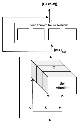
The input vector x is passed through a linear transformation layer which transforms the input into query q, key k, and value v vectors, given by the equations above. This is passed through a stacked multi-head self-attention layer which extracts global information across pairwise sequence of words to produce the output vector Z also given by the equation above. The equation for Z can be compared to how similarity is computed between the key and value pairs in databases. This output is added to the residual input x to preserve the meaning of individual words in addition to the pairwise representations. This is normalized to produce the output [math]\displaystyle{ \mathbf{(Z+x)} \in \mathbb{R}^{h \times r} }[/math]. This serves as the input to the feed forward neural network.

Feed Forward Neural Network

While the attention mechanism captures global information between words and hence aggregates across columns, the feed forward neural network aggregates across rows and takes a more broader look at each word independently. In a classroom environment, the attention mechanism is similar to the teacher observing the interactions among students in a group, whereas the feed forward neural network resembles the teacher evaluating each student independently for their understanding of the assignment. The output of the feed forward layer r also has a residual connection from the previous layer which is normalized and passed as the input of the decoder as (r+(z+x)). The encoder also has a positional encoding component which captures information about the position of words in a sequence.

While the above figure zooms in at how a word vector x is processed by the encoder, the major advantage of the transformer architecture is its ability to handle multiple words in a sequence parallely and so in practice, the above zoomed in version of the encoder is usually stacked to handle a group of words in parallel.