Graph Structure of Neural Networks
Presented By
Xiaolan Xu, Robin Wen, Yue Weng, Beizhen Chang
Introduction
During the study of Neural Networks, it is especially important to build a relation between a neural network’s accuracy and its underlying graph structure. The natural choice is to use computational graph representation but it has many limitations such as lack of generality and disconnection with biology/neuroscience.
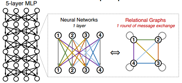
Thus, we develop a new way of representing a neural network as a graph, which we call a relational graph. Our key insight is to focus on message exchange, rather than just on directed data flow. For example, for a fixed-width fully-connected layer, we can represent one input channel and one output channel together as a single node, and an edge in the relational graph represents the message exchange between the two nodes. Under this formulation, using the appropriate message exchange definition, we show that the relational graph can represent many types of neural network layers.
We designed WS-flex, as a graph generator that allows us to systematically explore the design space of neural networks. We characterize neural networks by the clustering coefficient and average path length of their relational graphs under the insights of neuroscience.
Neural Network as Relational Graph
First, we define a graph [math]\displaystyle{ G =(V; E) }[/math] by its node set [math]\displaystyle{ V =\{v_1,...,v_n\} }[/math] and edge set [math]\displaystyle{ E \subseteq \{(v_i,v_j)|v_i,v_j\in V\} }[/math]. We assume that each node $v$ correpsonds with a feature [math]\displaystyle{ x_v }[/math], which might be scalar, vector or tensor quantity. All nodes have self edges, that is [math]\displaystyle{ (v_i,v_i)\in E }[/math], and the graph we consider here is undirected.
We call graph [math]\displaystyle{ G }[/math] a relational graph, when it is associated with message exchanges between neurons. (It is not necessary for one node in neural network to correspond with one node in the relational graph.) The association can be more complicated.
First: Graph
Second: Graph with Message Exchange
Message Exchange: Message Function + Aggregation Function
Round of Message Excnage
Specifically, a message exchange is defined by a message function and an aggregation function. A meesage function takes a node's feature [math]\displaystyle{ x_v }[/math] and then outputs an measage.
An aggregation function: taking a set of messages and then output the updated node feature. Basically the aggregation function descirbes the way how the message is combined.
At each round of message exchange, each node sends messages to its neighbors and aggregates incoming messages from its neighbors. This start to look like a neural network.
Each message is transformed at each edge through a message function [math]\displaystyle{ f(·) }[/math], then they are aggregated at each node via an aggregation function [math]\displaystyle{ AGG(·) }[/math]. Suppose we conduct [math]\displaystyle{ r }[/math] rounds of message exchange, then the [math]\displaystyle{ r^{th} }[/math] round of message exchange for a node [math]\displaystyle{ v }[/math] can be described as
where [math]\displaystyle{ \mathbf{x}^{(r+1)} }[/math] is the feature of of the [math]\displaystyle{ v }[/math] node in the relational graph after the [math]\displaystyle{ r^{th} }[/math] round of update. [math]\displaystyle{ u,v }[/math] are nodes in Graph [math]\displaystyle{ G }[/math]. [math]\displaystyle{ N(u)=\{u|(u,v)\in E\} }[/math] represents the set of all the neighbor nodes of [math]\displaystyle{ u }[/math].
A fixed-width MLP corresponds with a complete relational graph with a special message exchange function. Therefore, a fixed-width MLP is a special case under a much more general model family, where the message function, aggregation function, and most importantly, the relation graph structure can vary. The different relational graph represents the different topological structure and information exchange pattern of the network
Exploring and Generating Relational Graphs
We will deal with the design and how to explore the space of relational graphs in this section. There are three parts we need to consider:
(1) Graph measures that characterize graph structural properties:
We will use one global graph measure, average path length, and one local graph measure, clustering coefficient in this paper. To explain clearly, average path length measures the average shortest path distance between any pair of nodes; the clustering coefficient measures the proportion of edges between the nodes within a given node’s neighbourhood, divided by the number of edges that could possibly exist between them, averaged over all the nodes.
(2) Graph generators that can generate the diverse graph:
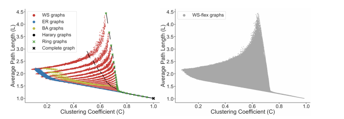
With selected graph measures, we use a graph generator to generate diverse graphs to cover a large span of graph measures. To figure out the limitation of the graph generator and find out the best, we investigate some generators including ER, WS, BA, Harary, Ring, Complete graph and results shows as below:
Thus, from the picture, we could obtain the WS-flex graph generator that can generate graphs with a wide coverage of graph measures; notably, WS-flex graphs almost encompass all the graphs generated by classic random generators mentioned above.
(3) Computational Budget that we need to control so that the differences in performance of different neural networks are due to their diverse relational graph structures.
It is important to ensure that all networks have approximately the same complexities so that the differences in performance are due to their relational graph structures when comparing neutral work by their diverse graph.
We use FLOPS (# of multiply-adds) as the metric. We first compute the FLOPS of our baseline network instantiations (i.e. complete relational graph) and use them as the reference complexity in each experiment. From the description in section 2, a relational graph structure can be instantiated as a neural network with variable width. Therefore, we can adjust the width of a neural network to match the reference complexity without changing the relational graph structures.
Experimental Setup
CIFAR-10 dataset: 10 classes, 50K training images and 10K validation images
ImageNet classification: 1K image classes, 1.28M training images and 50K validation images.
Discussions and Conclusions
Section 5 of the paper summarize the result of experiment among multiple different relational graphs through sampling and analyzing.
Neural networks performance depends on its structure
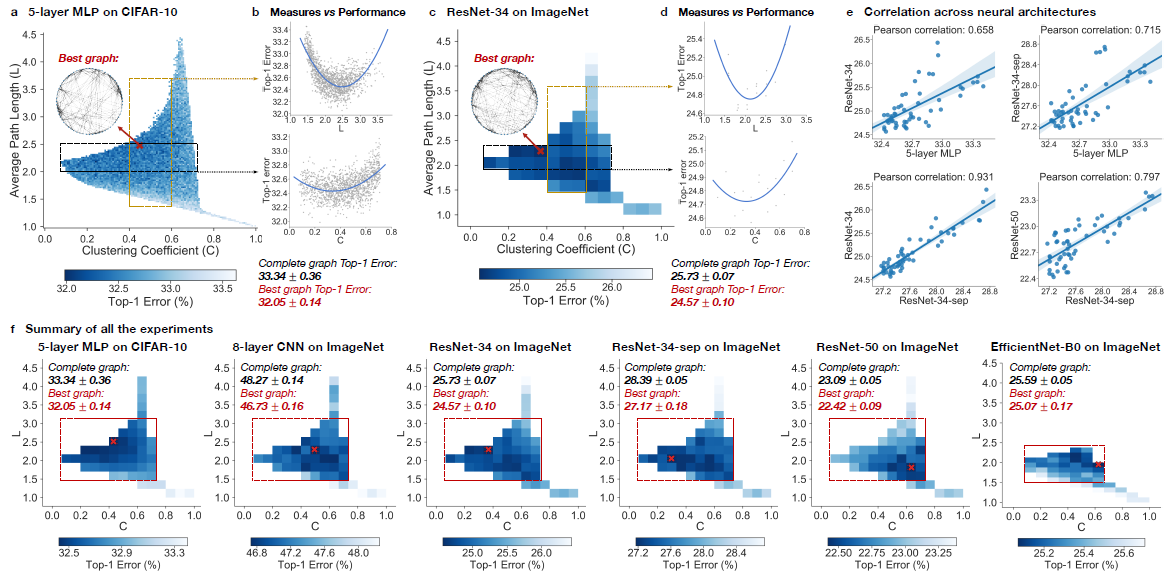
In the experiment, top-1 errors are going to be used to measure the performance of the model. The parameters of the models are average path length and clustering coefficient. Heat maps was created to illustrate the difference of predictive performance among possible average path length and clustering coefficient. In Figure ???, The darker area represents a smaller top-1 error which indicate the model perform better than other area. Compare with the complete graph which has A = 1 and C = 1, The best performing relational graph can outperform the complete graph baseline by 1.4% top-1 error for MLP on CIFAR-10, and 0.5% to 1.2% for models on ImageNet. Hence it is an indicator that the predictive performance of neural network highly depends on the graph structure, or equivalently that completed graph does not always preform the best.
Sweet spot where performance is significantly improved
To reduce the training noise, the 3942 graphs that in the sample had been grouped into 52 bin, each bin had been colored based on the average performance of graphs that fall into the bin. Based on the heat map, the well-performing graphs tend to cluster into a special spot that the paper called “sweet spot” shown in the red rectangle.
Relationship between neural network’s performance and parameters
When we visualize the heat map, we can see that there are no significant jump of performance that occurred as small change of clustering coefficient and average path length. If one of the variable is fixed in a small range, it is observed that a second degree polynomial is a good visualization tools for the overall trend. Therefore, both clustering coefficient and average path length are highly related with neural network performance by a U-shape.
Consistency among many different tasks and datasets
It is observed that the results are consistent through different point of view. Among multiple architecture dataset, it is observed that the clustering coefficient within [0.1,0.7] and average path length with in [1.5,3] consistently outperform the baseline complete graph.
Among different dataset with network that has similar clustering coefficient and average path length, the results are correlated, The paper mentioned that ResNet-34 is much more complex than 5-layer MLP but a fixed set relational graphs would perform similarly in both setting, with Pearson correlation of 0.658, the p-value for the Null hypothesis is less than 10^-8.
top architectures can be identified efficiently
According to the graphs we have in the Key Results. We can see that there is a "sweet spot" and therefore, we do not have to train the entire data set for a large value of epoch or a really large sample. We can take a sample of the data around 52 graphs that would have a correlation of 0.9 which indicates that fewer samples are needed for a similar analysis in practice. Within 3 epochs, the correlation between the variables is already high enough for future computation.
well-performing neural networks have graph structure surprisingly similar to those of real biological neural networks
The way we define relational graphs and average length in the graph is similar to the way information is exchanged in network science. The biological neural network also has a similar relational graph representation and graph measure with the best-performing relational graph.
Critique
1. The experiment is only measuring on a single data set which might impact the conclusion since this is not representative enough. 2. When we are fitting the model, training data should be randomized in each epoch to reduce the noise.


