User:Msikarou
Presented by
Milad Sikaroudi
Introduction
Transfer learning is a line of research in machine learning which focuses on storing knowledge from one domain (source domain) to solve a similar problem in another domain (target domain). In addition to regular transfer learning, one can use "transfer metric learning" in which through utilizing similarity relationship between samples [1], [2] a more robust and discriminative data representation is formed. However, both of these kinds of techniques work insofar as the domain shift, between source and target domains, is negligible. Domain shift is defined as the deviation in the distribution of the source domain and the target domain and it would cause the DNN model to completely fail. The multi-domain learning is the solution when the assumption of "source domain and target domain comes from an almost same distribution" may not hold. There are two variants of MDL in the literature that can be confused, i.e. domain generalization, and domain adaptation; however in domain adaptation, we have access to the target domain data somehow, while that is not the case in domain generalization. This paper introduces a technique for domain generalization based on two complementary losses that regularize the semantic structure of the feature space through an episodic training scheme originally inspired by the model-agnostic meta-learning.
Previous Work
Originated from model-agnostic meta-learning (MAML), episodic training has been vastly leveraged for addressing domain generalization [1, 26, 27, 31, 12, 28, 30, 34, 35]. The method of MLDG [26] closely follows MAML in terms of back-propagating the gradients from an ordinary task loss on meta-test data, but it has its own limitation as the use of the task objective might be sub-optimal since it only uses class probabilities. Most of the works [1,31] in the literature lack notable guidance from the semantics of feature space, which contains crucial domain-independent ‘general knowledge’ that can be useful for domain generalization. The authors claim that their method is orthogonal to previous works.
Model Agnostic Meta Learning
a.k.a learning to learn is a learning paradigm in which optimal initial weights are found incrementally (episodic training) by minimizing a loss function over some similar tasks (meta-train, meta-test sets). Imagine a 4-shot 2-class image classification task as below:
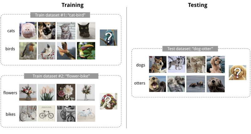
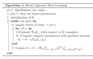
Each of the training tasks provides an optimal initial weight for the next round of the training. By considering all of these sets of updates and meta-test set, the updated weights are calculated using the below algorithm.
Method
Assume there are source domain [math]\displaystyle{ S }[/math] and T target domain [math]\displaystyle{ T }[/math]. We define a single model parametrized as [math]\displaystyle{ \theta }[/math] to solve the specified task. DG aims for training [math]\displaystyle{ \theta }[/math] on the source domains, such that it generalizes to the target domains. At each learning iteration we split the original S source domains [math]\displaystyle{ S }[/math] into S−V meta-train domains [math]\displaystyle{ \bar{S} }[/math] and V meta-test domains [math]\displaystyle{ \breve{S} }[/math] (virtual-test domain). This is to mimic real train-test domain-shifts so that over many iterations we can train a model to achieve good generalization in the final-test evaluated on target domains T .
The paper explains the method based on two approaches; Supervised Learning and Reinforcement Learning.
Supervised Learning
First, [math]\displaystyle{ l(\hat{y},y) }[/math] is defined as a cross-entropy loss function. ( [math]\displaystyle{ l(\hat{y},y) = -\hat{y}log(y) }[/math]). The process is as follows.
Meta-Train
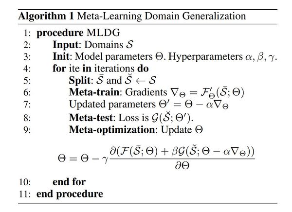
The model is updated on S-V domains [math]\displaystyle{ \bar{S} }[/math] and the loss function is defined as: [math]\displaystyle{ F(.) = \frac{1}{S-V} \sum\limits_{i=1}^{S-V} \frac {1}{N_i} \sum\limits_{j=1}^{N_i} l_{\theta}(\hat{y}_j^{(i)}, y_j^{(i)}) }[/math] In this step the model is optimized by gradient descent like follows: [math]\displaystyle{ \theta^{\prime} = \theta - \alpha \nabla_{\theta} }[/math]
Meta-Test
In each mini-batch the model is also virtually evaluated on the V meta-test domains [math]\displaystyle{ \breve{S} }[/math]. This meta-test evaluation simulates testing on new domains with different statistics, in order to allow learning to generalize across domains. The loss for the adapted parameters calculated on the meta-test domains is as follows: [math]\displaystyle{ G(.) = \frac{1}{V} \sum\limits_{i=1}^{V} \frac {1}{N_i} \sum\limits_{j=1}^{N_i} l_{\theta^{\prime}}(\hat{y}_j^{(i)}, y_j^{(i)}) }[/math]
the loss on the meta-test domain is calculated using the updated parameters [math]\displaystyle{ \theta }[/math] from meta-train. This means that for optimization with respect to [math]\displaystyle{ G }[/math] we will need the second derivative with respect to [math]\displaystyle{ \theta }[/math].
Final Objective Function
Combining the two loss functions, the final objective function is as follows: [math]\displaystyle{ argmin_{\theta} \; F(\theta) + \beta G(\theta - \alpha F^{\prime}(\theta)) }[/math]. Algorithm 1 illustrates the supervised learning approach.
Reinforcement Learning
In application to the reinforcement learning (RL) setting, we now assume an agent with a policy π that inputs states x and produces actions a in a sequential decision making task: [math]\displaystyle{ a_t = \pi_{\theta}(x_t) }[/math]. The agent operates in an environment and its goal is to maximize its return, [math]\displaystyle{ R = \sum\limits_{t} \delta^t R_t(x_t, a_t) }[/math]. Here, tasks map to return functions and domains map to different environments.
Meta-Train
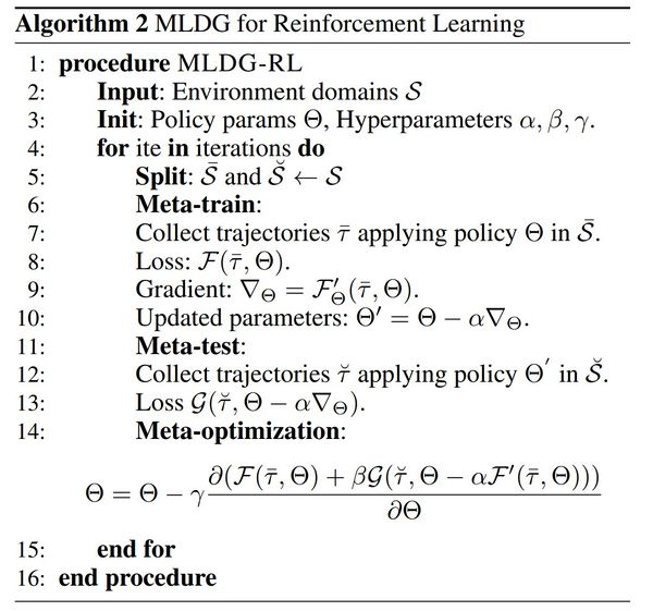
In meta-training, the loss function [math]\displaystyle{ F(·) }[/math]now corresponds to the negative return [math]\displaystyle{ R }[/math] of policy [math]\displaystyle{ \pi_{\theta} }[/math], averaged over all the meta-training environments in [math]\displaystyle{ \bar{S} }[/math].
Meta-Test
The step is like meta-test of supervised learning and loss is again negative of return function. For RL calculating this loss requires rolling out the meta-train updated policy <math> \theta in the meta-test domains to collect new trajectories and rewards. The reinforcement learning approach is also illustrated completely in algorithm 2.
Alternative Variants of MLDG
The authors propose different variants of MLDG objective function. For example the so-called MLDG-GC is one that normalizes the gradients upon update to compute the cosine similarity. It is given by: \begin{equation} \text{argmin}_\theta F(\theta) + \beta G(\theta) - \beta \alpha \frac{F'(\theta) \cdot G'(\theta)}{||F'(\theta)||_2 ||G'(\theta)||_2}. \end{equation}
Another one stops the update of the parameters after the meta-train has converged. This intuition gives the following objective function called MLDG-GN: \begin{equation} \text{argmin}_\theta F(\theta) - \beta ||G'(\theta) - \alpha F'(\theta)||_2^2 \end{equation}.
Experiments
The Proposed method is exploited in 4 different experiment results (2 supervised and 2 reinforcement learning experiments).
Illustrative Synthetic Experiment
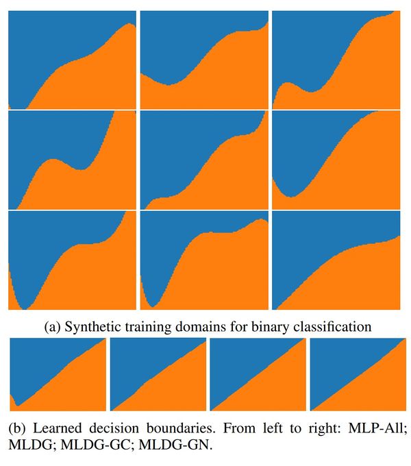
In this experiment, nine domains by sampling curved deviations are synthesized from a diagonal line classifier. We treat eight of these as sources for meta-learning and hold out the last for final-test. Fig. 1 shows the nine synthetic domains which are related in form but differ in the details of their decision boundary. The results show that MLDG performs near perfect and the baseline model without considering domains overfits in the bottom left corner.
Object Detection
For object detection, the PACS multi-domain recognition benchmark is exploited; a dataset designed for the cross-domain recognition problems .This dataset has 7 categories (‘dog’, ‘elephant’, ‘giraffe’, ‘guitar’, ‘house’, ‘horse’ and ‘person’) and 4 domains of different stylistic depictions (‘Photo’, ‘Art painting’, ‘Cartoon’ and ‘Sketch’). The diverse depiction styles provide a significant domain gap. The Result of Current approach compared to other approaches are presented in Table 1. The baseline models are D-MTAE[5],Deep-All (Vanilla AlexNet)[2], DSN[6]and AlexNet+TF[2]. On average, the Proposed method outperforms other methods.

Cartpole
The objective is to balance a pole upright by moving a cart. The action space is discrete – left or right. The state it has four elements: the position and velocity of cart and angular position and velocity of the pole. There are two sub-experiments designed. In the first one, domain factor is varied by changing the pole length. They simulate 9 domains with pole lengths. In the second they vary multiple domain factors – pole length and cart mass. In both experiments, we randomly choose 6 source domains for training and hold out 3 domains for (true) testing. Since the game can last forever, if the pole does not fall, we cap the maximum steps to 200. The result of both experiments are presented in Tables 2 and 3. The baseline methods are RL-All (Trains a single policy by aggregating the reward from all six source domains) RL-Random-Source (trains on a single randomly selected source domain) and RL-undo-bias: Adaptation of the (linear) undo-bias model of [7]. The proposed MLDG outperform the baselines.


Mountain Car
In this classic RL problem, a car is positioned between two mountains, and the agent needs to drive the car so that it can hit the peak of the right mountain. The difficulty of this problem is that the car engine is not strong enough to drive up the right mountain directly. The agent has to figure out a solution of driving up the left mountain to first generate momentum before driving up the right mountain. The state observation in this game consists two elements: the position and velocity of the car. There are three available actions: drive left, do nothing, and drive right. Here the baselines are the same as Cartpole. The model doesn't outperform the RL-undo-bias but has a close return value. The results are shown in Table 4.

Conclusion
This paper proposed a model-agnostic approach to domain generalization unlike prior model-based domain generalisation approaches, and it scales well with number of domains and it can also be applied to different Neural Network models. Experimental evaluation shows state-of-the-art results on a recent challenging visual recognition benchmark and promising results on multiple classic RL problems.
References
[1]: Koch, Gregory, Richard Zemel, and Ruslan Salakhutdinov. "Siamese neural networks for one-shot image recognition." ICML deep learning workshop. Vol. 2. 2015.
[2]: Hoffer, Elad, and Nir Ailon. "Deep metric learning using triplet network." International Workshop on Similarity-Based Pattern Recognition. Springer, Cham, 2015.
[3]: [Muandet, Balduzzi, and Scholkopf 2013] ¨ Muandet, K.; Balduzzi, D.; and Scholkopf, B. 2013. Domain generalization via invariant feature representation. In ICML.
[4]: [Ganin and Lempitsky 2015] Ganin, Y., and Lempitsky, V. 2015. Unsupervised domain adaptation by backpropagation. In ICML.
[5]: [Ghifary et al. 2015] Ghifary, M.; Bastiaan Kleijn, W.; Zhang, M.; and Balduzzi, D. 2015. Domain generalization for object recognition with multi-task autoencoders. In ICCV.
[6]: [Bousmalis et al. 2016] Bousmalis, K.; Trigeorgis, G.; Silberman, N.; Krishnan, D.; and Erhan, D. 2016. Domain separation networks. In NIPS.
[7]: [Khosla et al. 2012] Khosla, A.; Zhou, T.; Malisiewicz, T.; Efros, A. A.; and Torralba, A. 2012. Undoing the damage of dataset bias. In ECCV.