Deep Residual Learning for Image Recognition
Presented by
This report summary is presented by Hanzhen Yang, Jing Pu Sun, Ganyuan Xuan, Yu Su, Jiacheng Weng, Keqi Li, Yi Qian, and Bomeng Liu.
Introduction
Image recognition algorithms have seen tremendous advancement over the last decade thanks to the development of more powerful GPUs and the increasingly available data sets, two components essential to training of deep architectures. One of the more recent progresses in the field is the development of the Deep Residual Learning network, an expansion on the traditional neural network concretized by a group of researchers led by K. He from Microsoft Research. This impressive breakthrough was awarded first place in the ImageNet Large Scale Visual Recognition Challenge 2015 (ILSVRC 2015).
Any neural network is built under two main principles:
- Modularity: increase the depth of a network by simply repeating a small module and aim to achieve higher accuracy
- Residual learning: add a new layer to the existing network only if can get something extra from that additional layer
Based on these two principles, theoretically and given enough memory, neural networks may have as many layers as necessary. Yet, deeper networks possess two main problems:
- If the network is too deep, training errors may be hard to propagate back correctly. For example, even in the simplest scenario where the activation function is the identity mapping, training errors may still increase along the backpropagation.
- If the layers are too narrow, the neural network may not learn enough representation power. This results in the degradation problem when the network starts to converge: accuracy gets saturated then degrades rapidly.
To solve these two problems, K. He and his team developed the deep residual network algorithm, which allows deeper neural networks to be trained without sacrificing accuracy. This paper, “Deep Residual Learning for Image Recognition”, explains the concept of residual learning by first showcasing the structure of the network, followed by a comparison of experimental results to other models, and finally conclude with a discussion of some methodologies behind the network. In this report, we will attempt to explain this new methodology through our own words to ensure full understanding of the idea and exactly how it solved the issue of accuracy degradation.
Background
From all the techniques used for image classifications, deep neural networks are without doubt the current leaders in the category. A deep neural network (DNN) is an artificial neural network with multiple layers between the input and output layers, as opposed to a shallow neural network, which only has one layer of neurons. Through training, the deep neural network will find the optimal weights at each layer in order to transform the input data into output categories. Such algorithm can be applied to many fields, such as computer recognition of object through image classification. Such models can be trained by using image pixels information as numerical inputs and object that the image depicts as output. At every layer, outputs of the previous layer are applied a non-linear activation function and a linear transformation to finally output at the last layer one number corresponding to the category (class) as determined by the model. A neural network that contains many of such layers is called a deep neural network.
Since there are no limits on the number of neuron layers for a deep network, and due to the importance of the number of layers in the literature, a logical question follows: would the prediction accuracy of the model increase as we stack more layers? To answer this question, it is essential to inspect two main phenomenon that occur as the number of layers increase.
Vanishing/Exploding Gradients
A vanishing/exploding gradients is the problem of the partial derivative of the the error function going to 0 sometimes as the network stack up in layers. More precisely, when we perform backpropagation with gradient descent, each of the neural network’s weights increments proportionally to the partial derivative of the error function with respect to the current weight in each iteration of training. The error gradient with respect to weight parameters at shallower layers can be expressed as a chain rule expansion of parameters at deeper layers. When a network has large number of layers, the gradient tends to vanish or explode during back propagation.
Consider a simple example of feedforward neural network with only one neuron at each layer as shown in figure [XX1].
Figure [XX1]: simple feedforward neural network with one neuron at hidden layers
The error gradient of weight [math]\displaystyle{ w_1 }[/math] can be expressed as:
[math]\displaystyle{ \frac{\partial Err}{\partial w_1} = \frac{\partial Err}{\partial \hat{y}}\frac{\partial \hat{y}}{\partial x_3}\frac{\partial x_3}{\partial x_2}\frac{\partial x_2}{\partial w_1} \\ \ \ \ \ \ \ \ \ = \frac{\partial Err}{\partial \hat{y}} \cdot w_3 \cdot \sigma'(x_2 w_2) \cdot w_2 \cdot \sigma'(x_1 w_1) \cdot x_1 }[/math]
The activation function at each neuron is commonly selected to be Relu to avoid vanishing gradient when performing differentiation [REF]. When weight [math]\displaystyle{ w_3 }[/math] and [math]\displaystyle{ w_2 }[/math] are less than 1, the error gradient with respect to [math]\displaystyle{ w_1 }[/math] can be small due to multiplication of small numbers (a.k.a. vanishing gradient). When [math]\displaystyle{ w_3 }[/math] and [math]\displaystyle{ w_2 }[/math] are greater than 1, the error gradient with respect to [math]\displaystyle{ w_1 }[/math] can be large (a.k.a. exploding gradient). As the number of layers increases, the two cases of the problem are emphasized exponentially, reason for which deeper networks are difficult of training.
To address this problem, normalization layers was invented to enable networks with many layers to start converging for gradient descent with backpropagation.
Accuracy Degradation
A deep neural network that converges through training will likely encounter the second problem of accuracy degradation. As the number of layers increases, prediction accuracy becomes saturated and degrades rapidly beyond a certain number of layers (K.He, X.Zhang, S.Ren and J.Sun, 2016 ). Yet, this degradation is not due to overfitting. Experiments have shown that the training error increases as more layers are added to the model. The main reason behind this problem is the fact that different layers of the network learn at drastically different speed, which is also the reason why the initial model does not have a better performance than shallow network (M. Nielsen, 2013).
From empirical results, neural networks with stochastic gradient descent has difficulty optimizing the unnecessary weight to identity [1]. That is, adding more layers to a optimized model can increase the training error which contradicts to common understanding of neural networks. Figure [XX2] shows the comparison between training error of shallow and deep networks.
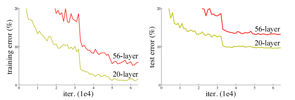
Based on the assumption that a deep neural network is capable of training identity weights when necessary, the DNN should not produce training error worse than shallower networks in any case. The previous example is thus a proof that the convolutional formulation of neural networks has difficulty of training identity.
A hypothetical model was then proposed based on this idea, one where the layers are copied from the learned shallower model and any additional layer would be weighted as the identity mapping. This hypothetical model should in theory have no worse performance than the founding shallower model. Yet, the Residual Neural Network presented here is a better approach to solve the problem of accuracy degradation.
Modeling
To resolve vanishing / exploding gradient and degradation of accuracy, residual network (Resnet) is proposed by K. He, etc [1]. The mathematical explanation are discussed in this section.
FIgure [XX3] shows a representation of Resnet building block. The main change of the Resnet is to include a short-cut that passes information directly from shallower layer to deeper layer.
Figure [XX3]: Residual learning: a building block [1]
Table [XX1] illustrates the comparison of training identity in a Resnet and a convolutional neural network. Relu operation of x is denoted as [math]\displaystyle{ f(x) }[/math]. Assuming x1 is the output of a previous building block, thus [math]\displaystyle{ ReLU(x_1) = x_1 }[/math]. In order to train identity in a Resnet building block, weight matrix need to be trained to 0 instead of I which is assumed to be easier[1]. This is further proven in the Experiment / Results section.
Table [XX1]: Comparison between no short-cut and with short-cut formulation
| Expression of [math]\displaystyle{ x_3 }[/math] | Condition for [math]\displaystyle{ x_1 = x_3 }[/math] | |
| No short-cut | [math]\displaystyle{ x_2 = f(W_2 \cdot f(W_1x_1)) }[/math] | [math]\displaystyle{ W_1 = W_2 = I }[/math] |
| With short-cut | [math]\displaystyle{ x_2 = f(W_2 \cdot f(W_1x_1) + x_1) }[/math] | [math]\displaystyle{ W_1 = 0 }[/math] or [math]\displaystyle{ W_2 = 0 }[/math] |
The formulation of Resnet also addresses the vanishing / exploding gradient problem. According to figure [XX3], we denote [math]\displaystyle{ F(x_1, W_1^{'}) = W_2 f(W_1x_1) }[/math] where [math]\displaystyle{ W_1^{'} }[/math] is the equivalent weight parameters, then [math]\displaystyle{ y_2 = x_1 + F(x_1, W_1^{'}), x_2 = f(y_2) }[/math]. To generalize the index, we obtain the following equations [3]:
[math]\displaystyle{ y_{l+1} = x_l + F(x_l, W_l^{'}) \\ x_{l+1} = f(y_{l+1}) }[/math]
Assuming [math]\displaystyle{ f }[/math] is identity, then recursively, we can express x at any deeper layer L using information from shallower layer as following [3]:
By rearranging equation above, and differentiating with chain rule, the following expression is obtained [3]:
[math]\displaystyle{ \frac{\partial Err}{\partial x_l} = \frac{\partial Err}{\partial x_L} \frac{\partial x_L}{\partial x_l} = \frac{\partial Err}{\partial x_L} (1+ \frac{\partial }{\partial x_l} \sum_{i=1}^{L-1} F(x_i, W_i^{'})) }[/math]
This suggests that the gradient at shallower layer [math]\displaystyle{ l }[/math] sees information directly from deeper layer [math]\displaystyle{ L }[/math]. To make the error gradient at layer [math]\displaystyle{ l }[/math] vanish, the derivative term of [math]\displaystyle{ \sum F }[/math]must be equal to -1 which is very difficult to achieve in a batch learning process [3]. Since error gradient with respect to [math]\displaystyle{ x_l }[/math] is part of back propagation process, preventing vanishing gradient wrt. [math]\displaystyle{ x_l }[/math] can effectively prevent vanishing gradient of [math]\displaystyle{ W_{l-1} }[/math].
Intuition of Resnet
Figure [XX4] shows a interesting way of understanding Resnet. By expanding a simple Resnet with 3 building block, a graph with all possible path of information is constructed. Therefore, the Resnet can also be seen as a majority voting process.
Figure [XX4]: Understand Resnet as a majority voting process [4]
Experimentation
To test the model, the authors of the paper applied it to the ImageNet 2012 dataset, which contains 1.28 million images for training, 50 000 for validation and 100 000 for testing. For comparison purposes, the team also ran two plain convolutional neural networks, one with 18-layers and one with 34-layers. Between the plain networks, the 34-layer plain network had a higher validation error than 18-layers plain throughout the training procedure. The team argues that this lack of accuracy is unlikely due to vanishing gradients, since the 34-layers network still expressed competitive accuracy compared to other image classification models. It was hypothesized that the fact that deep plain nets have exponentially low convergence rates relative to the number of layers is the main reason of the higher training error.

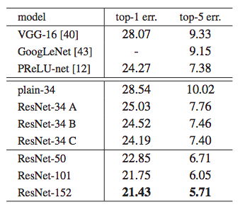
The team then tested two residual networks with same layers of neurons using the same dataset. Between the residual networks, 34-layers ResNet resulted in lower training error than the 18-layers ResNet during the entire training period. To further investigate the impact of projection shortcuts, 3 variations of the 34-layers model were built:
- zero padding shortcuts, all shortcuts are parameter-free,
- projection shortcuts other identity, and
- all projections.
As shown on the right, the result of the worst case with option B was better than option A, and C was slightly better than B. Nevertheless, the small difference in the 3 options concludes that the projection shortcuts are not essential for addressing the degradation problem.
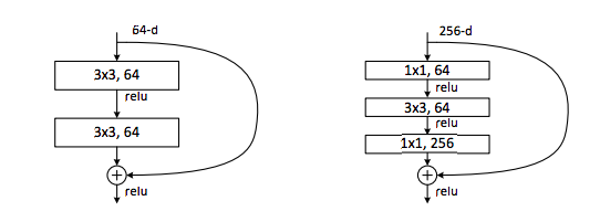
Due to concerns of training time constraints, the report then went on to test bottleneck designs, where the residual function uses 3 layers with increased dimension in the first and third layers rather than the previous 2 layers design, resulting in a 50-layers ResNet. (Left) The 1x1 convolutional layers are used to increase and decrease (restore) the dimensions, so that the middle 3x3 convolutional layer has smaller input/output dimensions. It important to emphasize on the identity shortcut here, since it was shown that another similar model with all projection shortcuts resulted in double time and complexity relative to option A. Even though the identity shortcut resulted in slightly higher error rate, its simple and fast design pattern outweighs the downside and it will be used for all bottleneck architectures.
CIFAR-10 10classes 50k training 10k testing
Focus on the behaviors of deep network. Inputs 32*32 images, per-pixel mean subtracted
1st layer 3*3 then use 6n layer with 3*3 on feature maps and 2n layers each feature map. Total have 6n +2 stacked weighted layers.
Use identity shortcuts in all cases => same depth width and number of parameters.
Weight decay 0.0001, momentum 0.9 use delving deep into rectifiers and batch normalization leaning rate 0.1. 32k,48k,64k iterations. Ref:24 traing. => 4 pixels pad on each side
Deep plain nets suffer from increased depth and exhibit higher training error when going deeper.(similar to ImageNet)
Change start to 0.01 learning rate till training error below 80% back to 0.1 learning rate. 110-layer converge well. Resnet have smaller responses than plain counterparts. => residual function generally closer to zero than non-residual functions. When using the 1000+layer, no optimization difficulty and have small training error. But the testing result is worse than 100+layer.(overfitting)
Appendix
VLAD
The area of image recognition and object retrieval has seen a steady trend of improvements in performance, where one of the most significant contribution is the introduction of the Vector of Locally Aggregated Descriptors (VLAD). It is designed to fit very large image datasets (e.g. 1 billion images) into main memory with its low dimension (e.g. 16 byte per image). https://www.robots.ox.ac.uk/~vgg/publications/2013/arandjelovic13/arandjelovic13.pdf
Fisher Vector
The Fisher Vector is an image representation obtained by sampling local image features, fitting Gaussian Mixture Model on those features, and resulting in vocabulary of dominant features in the image and their distributions. Form each Gaussian distribution, we measure the expectation of distance of image features using the likelihood a feature belongs to certain Gaussian. Concentrating result vector of each vocabulary into one large descriptor vector, normalize it, we will get the Fisher Vector. https://jacobgil.github.io/machinelearning/fisher-vectors-python
Multigrid Method
Multigrid Methods are algorithms for solving differential equations using a hierarchy of discretization. The main idea is to accelerate the convergence of basic iterative method with three significant strategies: smoothing, restriction and interpolation/prolongation. Which are used to reduce high frequency errors, down-sample the residual error to a coarser grid, and interpolate a correction computed on a coarser grid into a finer grid, respectively. https://www.wias-berlin.de/people/john/LEHRE/MULTIGRID/multigrid.pdf
VGG
VGG refers to a deep convolutional network for object recognition developed and trained by Oxford’s renowned Visual Geometry Group. VGGNet scored 1st place on image localization task and 2nd place on image detection task in the Image Net Large Scale Visual Recognition Challenge (ILSVRC) in 2014. VGG-16 network architecture and its python code listed below. https://gist.github.com/baraldilorenzo/07d7802847aaad0a35d3#file-vgg-16_keras-py
ReLU
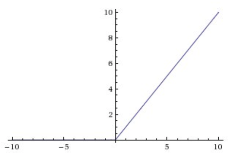
The Rectified Linear Unit (ReLU) is one of the most commonly used activation function in deep learning models. It is a non-negative function which returns 0 if the input is less than 0 and return the input itself otherwise. It can be written as f(x)=max(0,x) . Graphically it looks like
https://www.kaggle.com/dansbecker/rectified-linear-units-relu-in-deep-learning
Convolutional Neural Network (CNN)
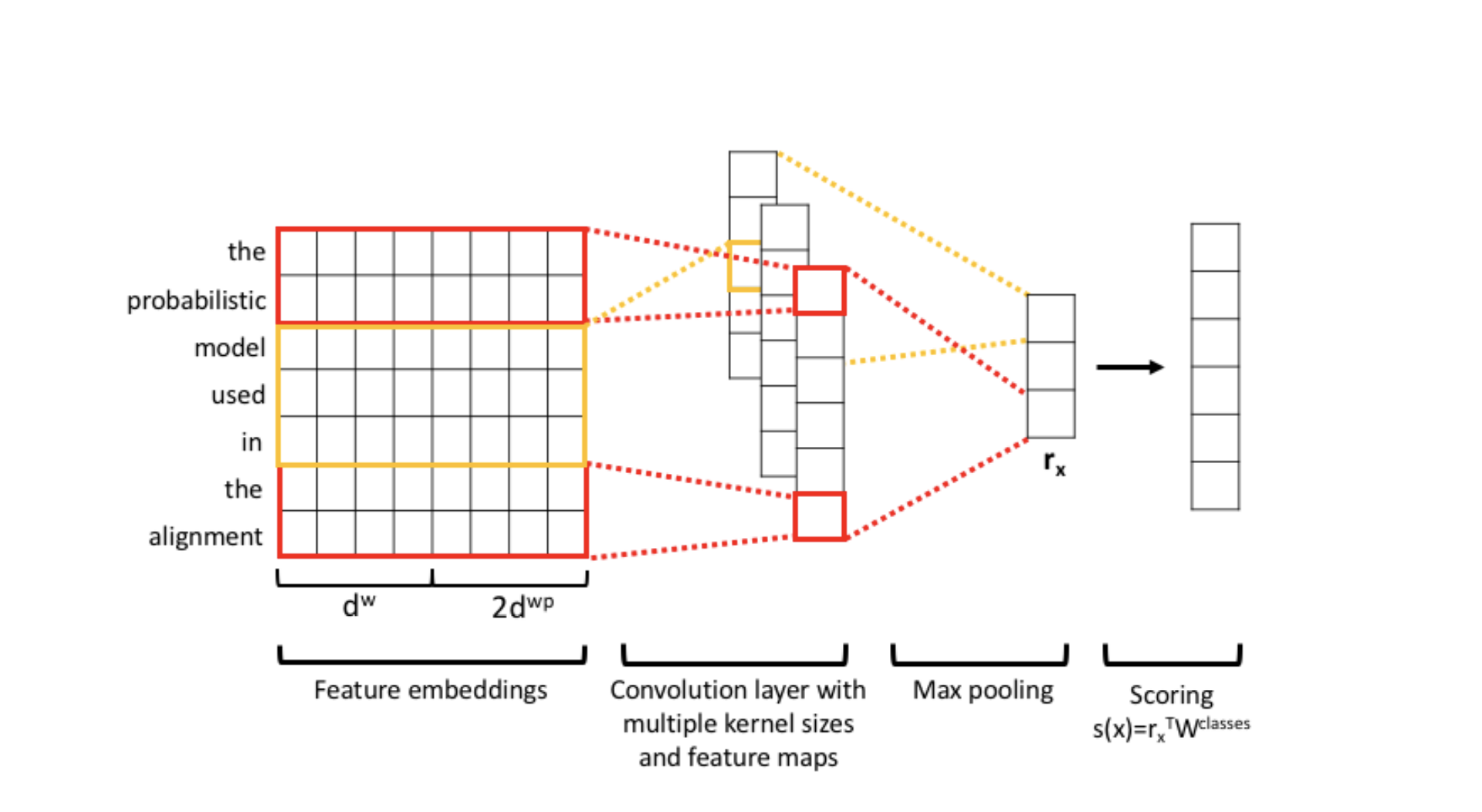
CNN is similar to ordinary neural networks that are made up of neurons with learnable weights and biases. Each of the neurons receives some inputs, performs a linear transformation and follows with a non-linear activation function. The difference is that CNN allow us to encode certain properties into the architecture since the explicit assumption is the inputs are images. A regular neuron receive a single vector as its input, which means a matrix input will be vectorized into a single column and achieve full connectivity. It will boost the number of parameters and lead to overfitting. CNN have neurons arranged in 3 dimensions: height, width and depth. The neurons in a layer will only be connected to a necessary portion of the layer before it, instead of wasteful fully connection. This will make CNN achieve higher accuracy and efficiency when dealing with image recognitions comparing to the ordinary neural network. A visualization is:
Left: A regular Neural Network. Right: A CNN arranges its neurons in three dimensions (width, height, depth). http://cs231n.github.io/convolutional-networks/
CIFAR-10
The CIFAR-10 is an established computer-vision dataset used for image recognition. It consists of 60000 32x32 color images which split into 10 completely mutually exclusive classes evenly. There are 50000 training images and 10000 test images. It is widely used in image recognition competitions and tasks.
References
- [1] K.He, X.Zhang, S.Ren and J.Sun. Deep Residual Learning for Image Recognition. 2016.
- [2] M.Nielsen.(2013). Neural Networks and Deep Learning.
- [3] K.He, X.Zhang, S.Ren and J.Sun. Identity Mappings in Deep Residual Networks. 2016.
- [4] A. Veit, M. Wilber, S. Belongie. Residual Networks Behave Like Ensembles of Relatively Shallow Networks. 2016.
- [5] Chen, Z. How does deep residual learning work? 2017.


